We'll discuss another gaseous
pollutant today, tropospheric ozone.
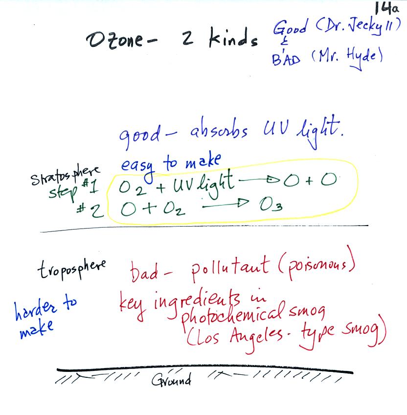
Ozone has a Dr. Jekyll and Mr. Hyde
personality. Ozone
in
the stratosphere (the ozone layer) is beneficial, it absorbs dangerous
high
energy ultraviolet light (which would otherwise reach the ground and
cause skin cancer, cataracts, and many other problems).
Ozone in the troposphere is bad, it is a pollutant. That is the stuff we will be concerned with today. Tropospheric ozone is also a key component of photochemical smog (also known as Los Angeles-type smog)
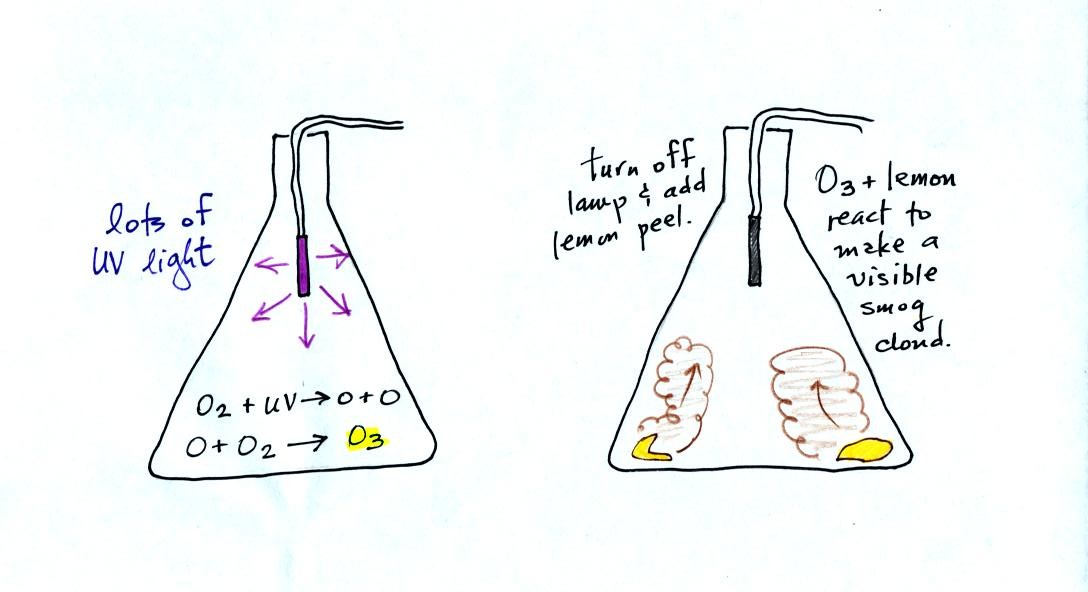
We'll be making some photochemical smog as a class demonstration. This will require ozone (and a hydrocarbon of some kind). We'll use the simple stratospheric recipe (equation above circled in yellow) for making ozone in the demonstration rather than the more complex tropospheric process (4-step process shown below).
Ozone in the troposphere is bad, it is a pollutant. That is the stuff we will be concerned with today. Tropospheric ozone is also a key component of photochemical smog (also known as Los Angeles-type smog)
We'll be making some photochemical smog as a class demonstration. This will require ozone (and a hydrocarbon of some kind). We'll use the simple stratospheric recipe (equation above circled in yellow) for making ozone in the demonstration rather than the more complex tropospheric process (4-step process shown below).
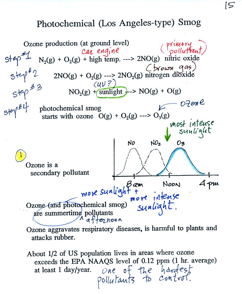
At the top of this figure you see that a more complex series of reactions is responsible for the production of tropospheric ozone. The production of tropospheric ozone begins with nitric oxide (NO). NO is produced when nitrogen and oxygen in air are heated (in an automobile engine for example) and react. The NO can then react with oxygen to make nitrogen dioxide, the poisonous brown-colored gas we made in class. Sunlight can dissociate (split) the nitrogen dioxide molecule producing atomic oxygen (O) and NO. O and O2 react in a 4th step to make ozone (O3). Because ozone does not come directly from an automobile tailpipe or factory chimney, but only shows up after a series of reactions, it is a secondary pollutant. Nitric oxide would be the primary pollutant in this example.
NO is produced early in the day (during the morning rush hour). The concentration of NO2 peaks somewhat later. Peak ozone concentrations are usually found in the afternoon. Ozone concentrations are also usually higher in the summer than in the winter. This is because sunlight plays a role in ozone production and summer sunlight is more intense than winter sunlight.
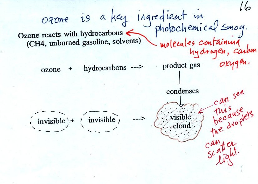
As shown in the figure below, invisible ozone can react with a hydrocarbon of some kind which is also invisible to make a product gas. This product gas sometimes condenses to make a visible smog cloud or haze. The cloud is composed of very small droplets or solid particles. They're too small to be seen but they are able to scatter light - that's why you can see the cloud.
The class demonstration of
photochemical smog is summarized
below (a flask was used instead of the aquarium shown on the bottom of
p. 16 in the photocopied class notes). We begin by using the UV
lamp to create and fill the flask with
ozone. Then a few pieces of fresh lemon peel were added to the
flask. A whitish cloud quickly became visible (colored brown in
the figure below).
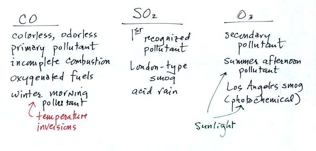
So here's a short recap: key
characteristics of the 3 pollutants we've talked about so far.
The last
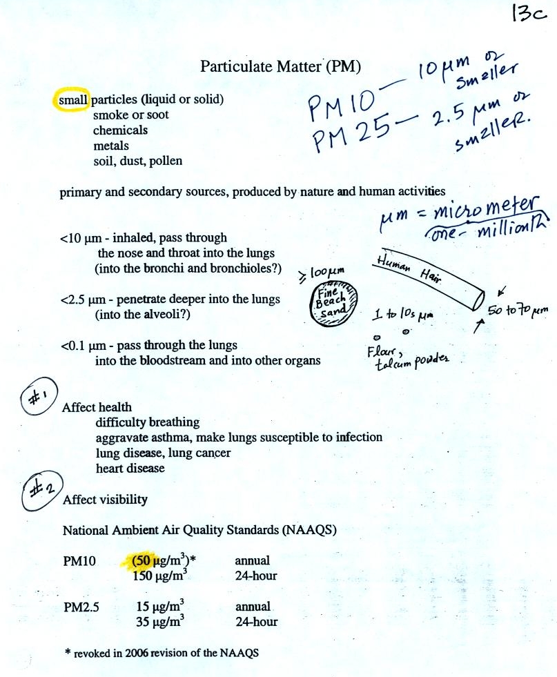
pollutant that we will cover is Particulate Matter (PM) - small solid
particles or drops of liquid (but not gas) that remain suspended in
the air (sometimes refer to as aerosols). The designations PM10
and PM25 refer to particles with
diameters less than 10 micrometers and 2.5 micrometers,
respectively. A micrometer is one millionth of a meter. The
drawing below might give you some idea of what a 1 micrometer particle
would look like (actually it would probably be too small to be seen
without magnification).
Particulate matter can be produced
naturally (wind blown dust,
clouds above volcanic eruptions, smoke from lightning-caused forest and
brush fires). Human activities also produce particulates.
Particles with dimensions of 10 micrometers and less can be inhaled into the lungs (larger particles get caught in the nasal passages). Inhaled particulates are a health threat. The particles can cause cancer, damage lung tissue, and aggravate existing repiratory diseases. The smallest particles can pass through the lungs and get into the blood stream (just as oxygen does) and damage other organs in the body.
The figure below identifies some of the parts of the human lung mentioned in the figure above.
 Crossectional view of the
human lungs
from: http://en.wikipedia.org/wiki/Lung |
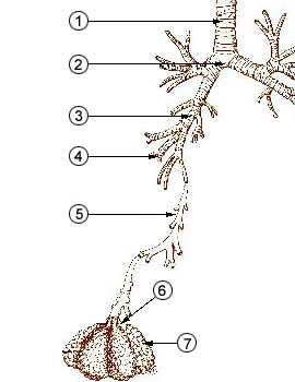 1 - trachea
from http://en.wikipedia.org/wiki/Image:Illu_quiz_lung05.jpg2 - mainstem bronchus 3 - lobar bronchus 4 - segmental bronchi
5 - bronchiole6 - alveolar duct 7 - alveolus |
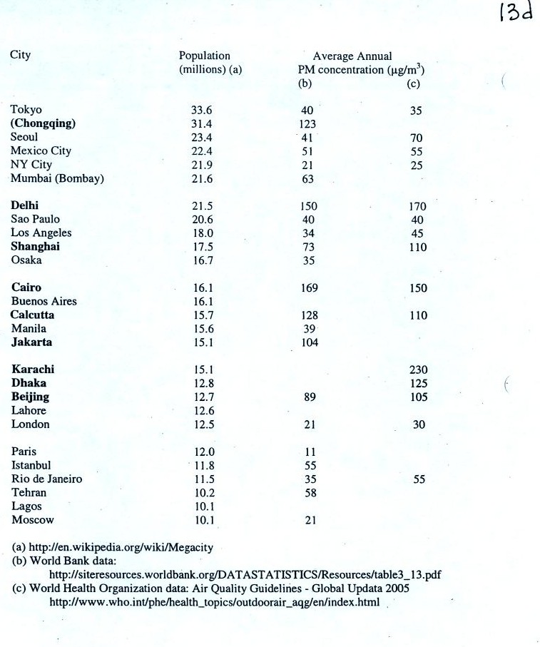
Note the PM10 annual National Ambient Air Quality Standard (NAAQS) value of 50 micrograms/meter3 at the bottom of p. 13c in the photocopied ClassNotes (above). The following list shows that there are several cities around the world where PM concentrations are 2 or 3 times higher than the NAAQS value.
There was some concern last summer
that the polluted air in
Beijing would keep athletes from performing at their peaks during the
Olympic
Games. Chinese authorities restricted transportation and
industrial activities both before and during the games in an attempt to
reduce pollutant concentrations. Rainy weather during the games
may have had the greatest effect, however. Clouds were mentioned but the figure
below was not shown in class.
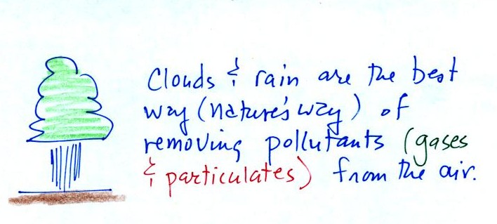
Clouds and precipitation are the
best way of cleaning pollutants from the air.
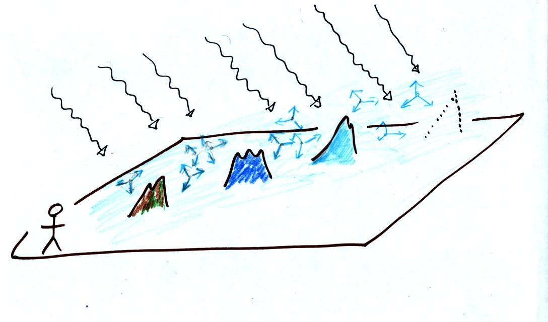
Particulates can affect visibility and can make the sky appear hazy. To understand this we need to look at how air molecules and particles scatter sunlight.
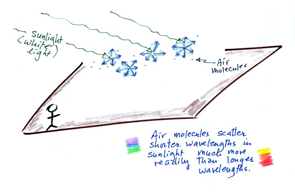
Air molecules scatter
sunlight (an individual air molecule doesn't scatter much light, but
there are lots of air molecules in the atmosphere). Sunlight is
basically white, which tells you it is a mixture of all the
colors. Because air molecules are small (relative to the
wavelength of visible light) they scatter shorter wavelengths more
readily than longer wavelengths. When you look away from the sun
and toward the sky you see this scattered light, it has a deep blue
color. This is basically why the sky is blue. If the earth
didn't have an atmosphere (or if air molecules didn't scatter light)
the sky would be black.
Scattering of sunlight by air molecules turns distant mountains blue and eventually makes them fade from view
A nearby mountain might appear dark green or brown. You are mostly seeing light reflected off the mountain. As the mountain gets further away you start seeing increasing amounts of blue light (sunlight scattered by air molecules in between you and the mountain) being added to the brown and green reflected light. As the mountain gets even further the amount of this blue light from the sky increases. Eventually the mountain gets so far away that you only see blue sky light and none of the light reflected by the mountain itself.
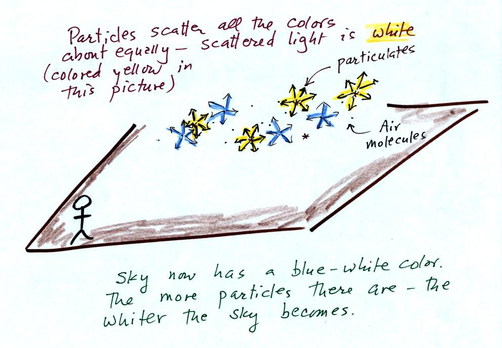
Particles also scatter light
(remember the chalk dust used in the laser demonstration).
But because the particle size is about equal to or somewhat greater
than the wavelength of visible light the particles scatter all the
colors equally. The light scattered by particles is white.
This is basically why clouds are white.
As the amount of particulate matter in the air increases the color of the sky changes from deep blue to whitish blue. The higher the particle concentration, the whiter the sky becomes.
I didn't explain the effect of particulates on visibility very well in the MWF class. I went back to my office, banged my head against the wall a few times, and tried to come up with a new approach. I'll try the following explanation on you T Th people.
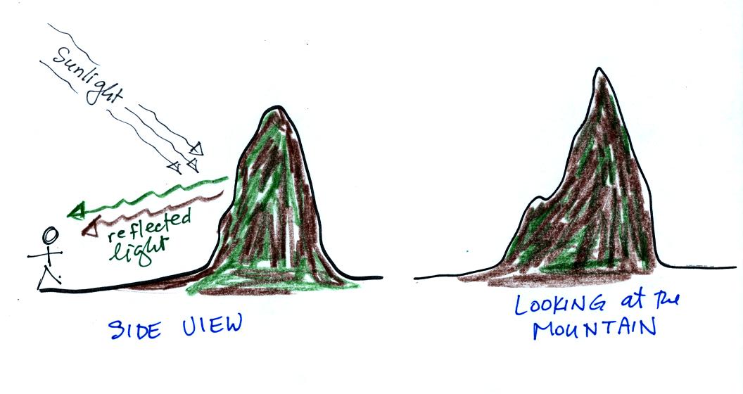
The air is free of particles in this first picture. You're looking at a relatively nearby mountain. The "side view" at left explains that you are able to see the mountain because it reflects sunlight back toward you. The picture at right is what you see when you look at the mountain.
As the amount of particulate matter in the air increases the color of the sky changes from deep blue to whitish blue. The higher the particle concentration, the whiter the sky becomes.
I didn't explain the effect of particulates on visibility very well in the MWF class. I went back to my office, banged my head against the wall a few times, and tried to come up with a new approach. I'll try the following explanation on you T Th people.
The air is free of particles in this first picture. You're looking at a relatively nearby mountain. The "side view" at left explains that you are able to see the mountain because it reflects sunlight back toward you. The picture at right is what you see when you look at the mountain.
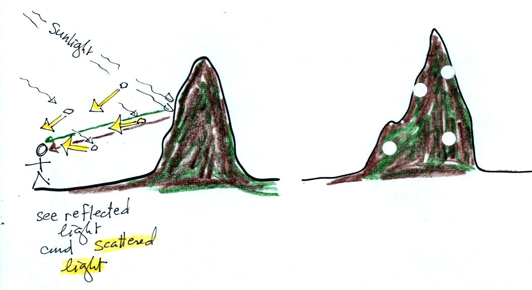
Now some particulates have been
added to the air. They scatter sunlight, the scattered light is
white (it's highlighted in yellow in the picture at left for
emphasis). So now you still see the brown and green reflected
light but also some white scattered light. Some (fairly big)
spots of white light have been added to the picture at right.
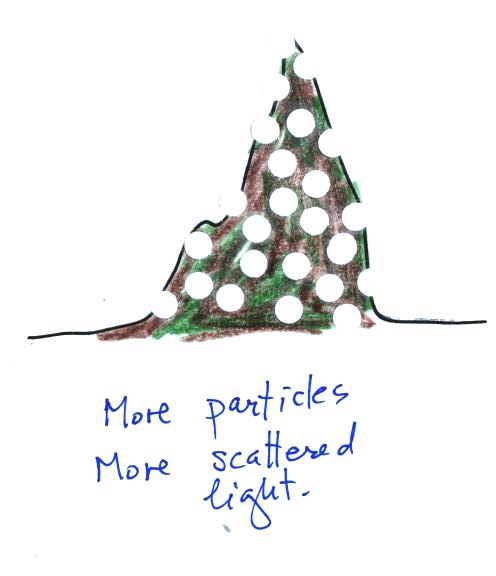
More particles have been added to
the air. That means there will be more scattered light.
We'll add even more particles to the air in the next picture. Because there is more scattered light (more spots of white light in the picture of the mountain) you have a harder time seeing the mountain.
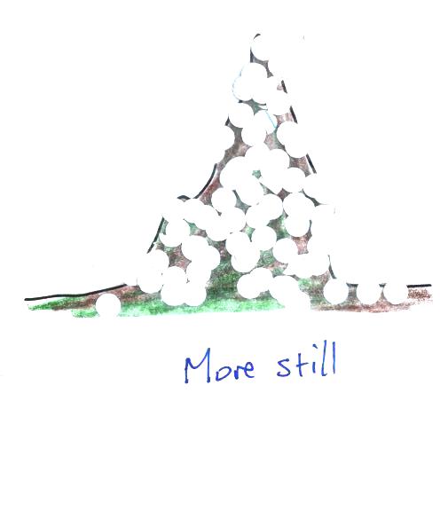
It's getting harder and harder to see the mountain.
We'll add even more particles to the air in the next picture. Because there is more scattered light (more spots of white light in the picture of the mountain) you have a harder time seeing the mountain.
It's getting harder and harder to see the mountain.
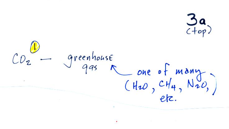
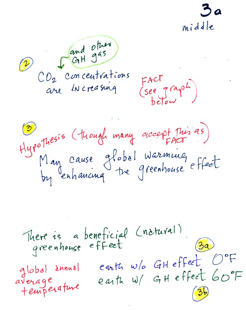
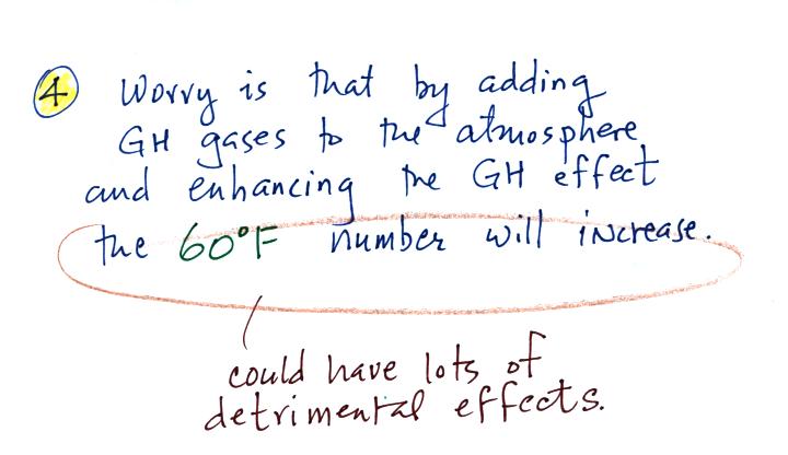
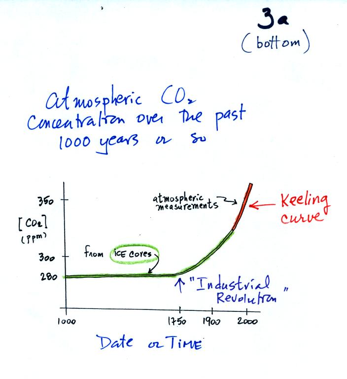
We spent the last part of the period today and will spend much of next Tuesday looking at the current concern over increasing greenhouse concentrations in the earth's atmosphere, global warming, and climate change. This is a big, complex, and contentious subject and we will only scratch the surface. I've reorganized the material presented in class into what is hopefully a much clearer introduction to this topic.
Quite a bit of information needs to be added to p. 3a in the photocopied ClassNotes; we will break it up into several smaller pieces.