Tuesday Feb. 14, 2006
Optional Assignment #2 was collected in class. A handout
with
answers to the questions was distributed together with the Quiz #1 Study Guide (Quiz #1 is Thursday,
Feb. 16, and will cover material on both Quiz #1 Study Guide and the Practice Quiz Study Guide). Some additional comments on the optional
assignment also available online.
The Experiment #1 reports are graded and can be picked up from the
instructor. Revised Expt. 1 reports are
due on Tues, Feb. 28. Please include the original report if you
turn in a revised report. You do not need to rewrite your entire
Expt. 1 report, only the portions where you hope to earn additional
credit.
The Expt. #2 reports are also due on Feb. 28. Though you should
be trying to collect your data now so that you can return the materials
and pick up the supplementary information sheet.
A time lapse video recording of a cold front passing through Tucson on
Easter Sunday in 1999 was shown in class.
The
following figure (from p. 41 in the photocopied notes) shows some of
the relationships that exist between surface and upper level weather
map features
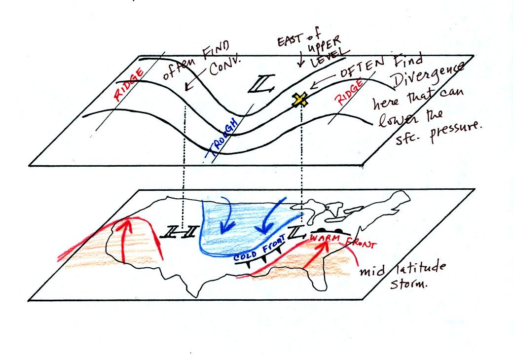
On the surface map you see centers of HIGH and LOW
pressure.
The low pressure center, together with the cold and warm fronts, is a
middle latitude storm. A storm of this type is what brought the
stormy weather to the east coast of the US this past weekend.
Note how the counterclockwise winds spinning around the LOW move warm
air northward (behind the warm front on the eastern side of the LOW)
and cold air southward (behind the cold front on the western side of
the LOW). Clockwise winds spinning around the HIGH also move warm
and cold air.
Note the ridge and trough features on the upper level chart. We
learned that warm air is found below an upper level ridge. Now
you can begin to see the source of this warm air. Warm air is
found west of the HIGH and to the east of the LOW. This is
where the two ridges on the upper level chart are also found. You
expect to find cold air below an upper level trough. This cold
air is being moved into the middle of the US by the northerly winds
that are found between the HIGH and the LOW.
Note the X marked on the upper level chart directly above the
surface LOW. This is a good location for a surface LOW to develop
and strengthen. The next figure (from p. 42 in the photocopied
notes) will give you some idea of why
this is true.
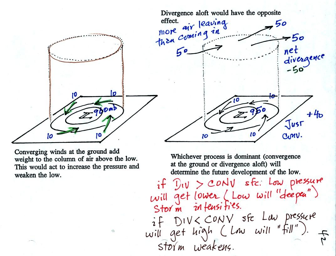
We'll start with the figure at left. We see a surface LOW
(with 960 mb
pressure drawn in as an example). Winds are spinning
counterclockwise and spiraling in
toward (converging) the center of the low. These surface winds
are moving air into the column of air and (as explained on the figure)
should cause the pressure in the center of the LOW to increase.
Imagine that each arrow brings in enough air to increase the pressure
at the center of the LOW by 10 mb. You would expect the pressure
at the center of the LOW to increase from 960 mb to 1000 mb. What
if the central pressure actually decreased? How would you explain
that?
This is just like a bank account. You have $960 in the bank and
make four $10 dollar deposits. You would expect your bank account
balance to increase from $960 to $1000. What if your account
balanced dropped? How would you explain that?
The right hand figure shows what is going on. We haven't included
the effects of addition and removal of air at upper levels.
Imagine that 50 mb worth of air are added to the column and 50+50=100
mb worth of air are removed. That's a net removal (net
divergence) of 50 mb.
So now we have 40 mb worth of air being added at the ground (surface
convergence) and 50 mb worth being removed at upper levels (upper level
divergence). The grand total is 10 mb of removal. The
surface pressure will decrease slightly.
You can apply the numbers in the right hand picture to the bank account
problem. You have $960 in the bank and make four $10
deposits.
However you also deposit $50 dollars and make two $50 withdrawals (the
top of the picture). That's a total of $90 being deposited and
$100 being withdrawn. Your bank account goes down $10.
In a case like this where upper
level divergence > surface convergence, the surface LOW
pressure will get even lower (the low will "deepen") and the storm will
strengthen. Click here if
you dare and if you would like to see what could happen next.
The other possibility is that the upper level divergence <
surface convergence. In this case the LOW pressure will
increase (the low will "fill") and the storm will weaken.
Click here for some additional
examples. By working through some additional examples you might
increase your understanding of this material and build up your
confidence (of course there's always a chance that more examples will
just make this topic more confusing - the choice is yours)
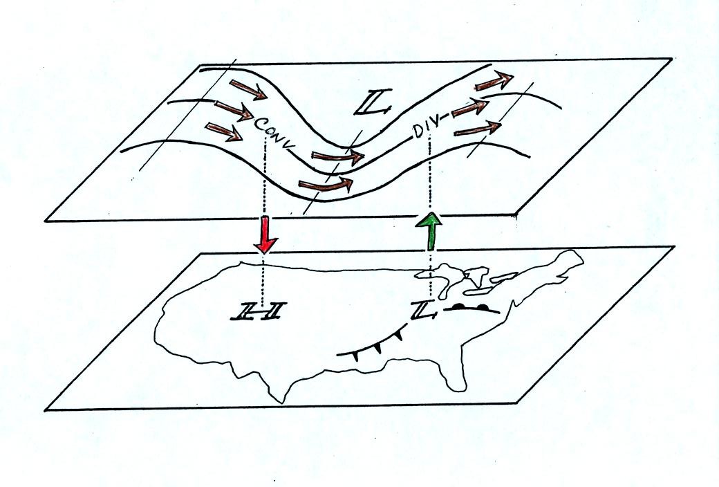
Now that you
have some idea of what upper level divergence looks like
you are in a position to understand another one of the relationships
between the surface and upper level winds.
One of the things we have learned about surface LOW pressure is that
the converging surface winds create rising air motions. The
figure above gives you an idea of what can happen to this rising air
(it has to go somewhere). Note the upper level divergence in the
figure: two arrows of air coming into the point "DIV" and three arrows
of air leaving (more air going out than coming in is what makes this
divergence). The rising air can, in effect, supply the extra
arrow's worth of air.
Three arrows of air come into the point marked "CONV" on the upper
level chart and two leave (more air coming in than going out).
What happens to
the extra arrow? It sinks, it is the source of the sinking air
found above surface high pressure.
Now
believe it or not we are going to move into Chapter 2. Here is a
short introduction to some of the material we will be covering (pps 43
& 44) in the photocopied notes.
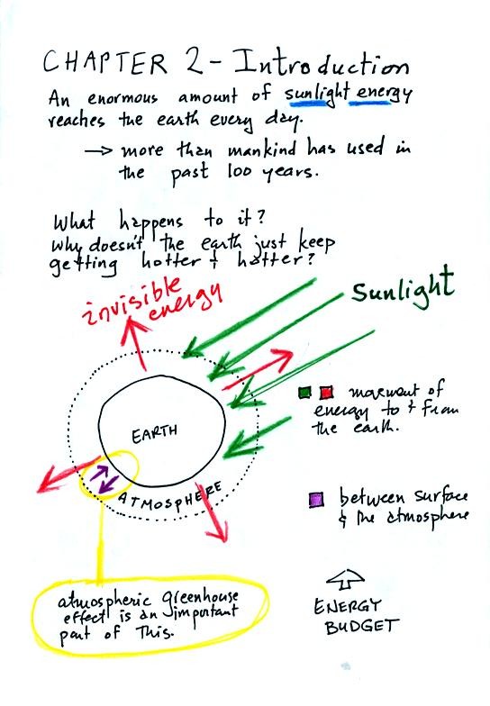
An enormous amount of sunlight energy reaches the earth everyday.
We will learn how it is possible for this form of energy to travel
through empty space. We'll also find that sunlight consists of a
little Ultraviolet light (~7%), Visible light (44%), and Infrared light
(48%) [the remaining 1% is composed of microwaves, radiowaves and
things like that]. With all of this energy arriving at and being
absorbed by the earth, what keeps the earth from getting hotter and
hotter? The answer is that the earth also sends energy back into
space (an invisible form of energy - infrared light). A balance
between incoming and outgoing energy is achieved and the earth's annual
average temperature remains constant.
We will also look closely at energy transport between the earth's
surface and the atmosphere. That is where the atmospheric
greenhouse operates. That will be a major goal in Chapter 2 - to
understand the atmospheric greenhouse effect.
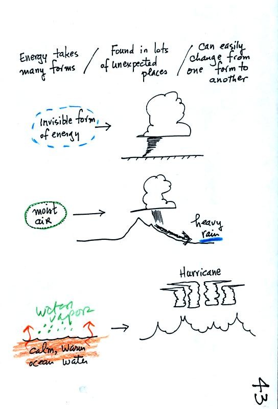
Water vapor is a particularly important form of invisible energy.
When water vapor condenses to produce the water droplets that produce a
cloud an enormous amount of energy is released into the atmosphere.
You can imagine the work that you would do carrying a gallon of water
(8 pounds) from Tucson to the top of Mt. Lemmon. To accomplish
the same thing Mother Nature must first evaporate the water and (if my
calculations are correct) that requires about 100 times the energy
needed to carry the 8 pounds of water to the summit of Mt.
Lemmon. And Mother Nature transports a lot more than just a
single gallon.
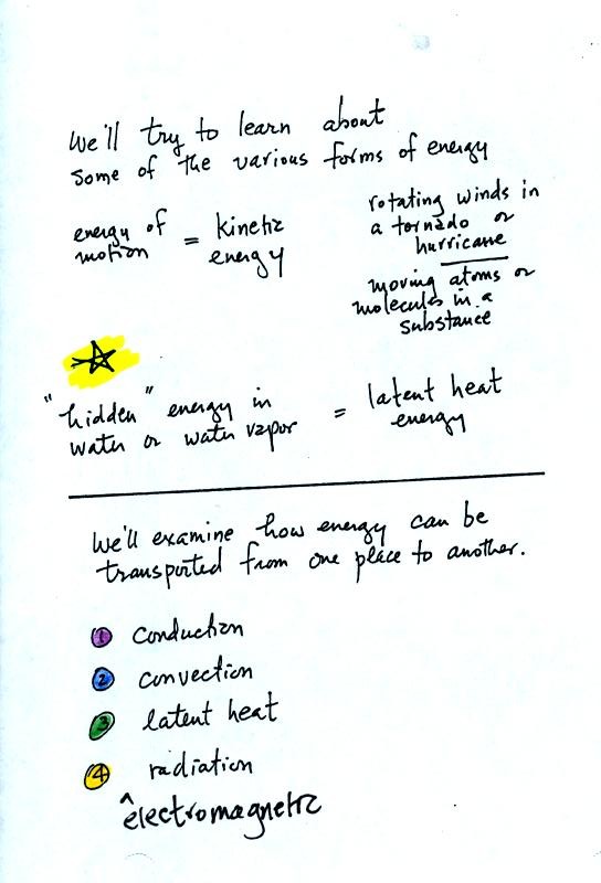
Kinetic energy is energy of motion. The four energy transport
processes are listed at the bottom of the page above. By far the
most important process is electromagnetic radiation. This is the
only process that can transport energy through empty space.
Somewhat surprisingly latent heat is the second most important
transport process.
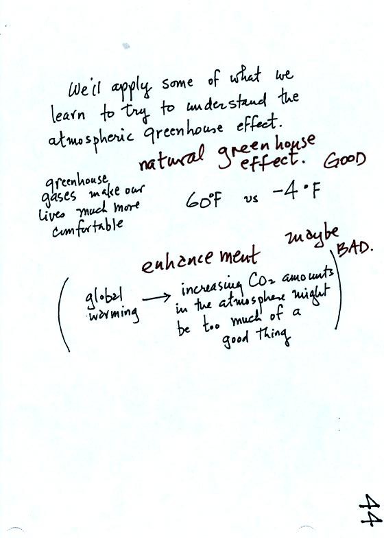
One of the main objectives in Chapter 2 to understand the greenhouse
effect.
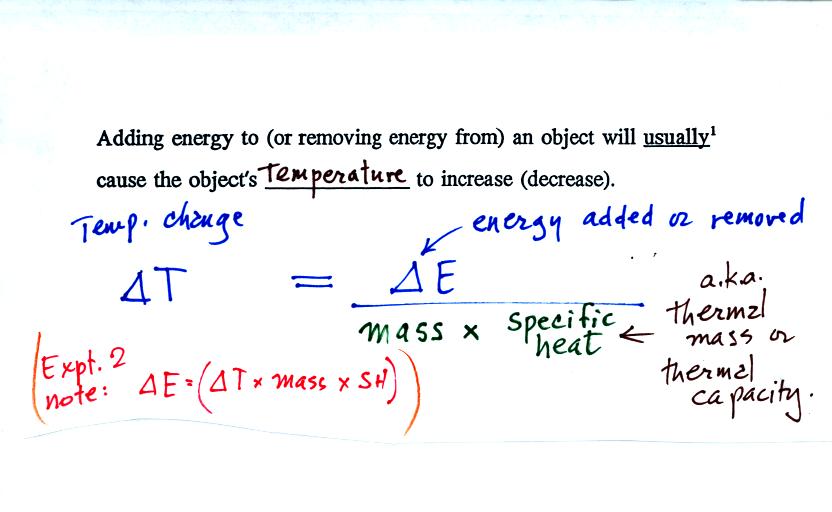
From the top of p. 47 in the photocopied notes: if you add
energy to
(or remove energy from) and object the object will usually warm up (or
cool off if you remove energy).
We need to come up with an equation that tells us exactly how much of a
temperature change there will be. The temperature change will
first depend on the amount of energy added (or removed).
If you add equal amounts of energy to a small rock and a
large rock,
the small rock will warm up more than the large rock. If you
place small and large pans of water on equal sized stove burners, the
small pan will heat up more quickly than the large pan of water.
These examples tell us that the temperature change depends on the
amount of material being heated (or cooled). The mass (not the
volume) should appear in the denominator of the equation.
There is one last term, the specific heat. The
specific heat is sometimes
called the thermal mass. An material with large specific heat
will warm or cool slowly when energy is added or removed (just as an
object with large mass would warm or cool slowly).
Note the slightly different form of the equation in
parenthesis. You can measure
the amount of energy added to or removed from a material of known mass
and specific heat by measuring the change in the object's
temperature. This relationship is used in Experiments 2 and 3.
Now we'll look at an
important example:
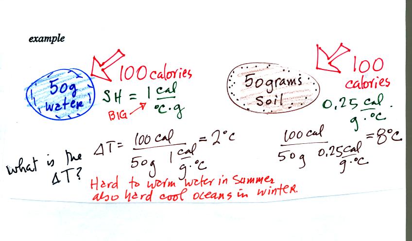
We add equal amounts of energy (note calories are units of energy) to
equal masses of water and soil. Water has a relatively high
specific heat and warms less than the soil. These two materials
were used in the example because the surface of the earth is made up of
water (oceans) and soil. Oceans moderate the climate. It is
hard to warm the ocean in the summer and hard to cool the ocean in the
winter. A city near an ocean will have less annual swing in
temperature than a city located in the middle of land mass.
Adding or removing energy will usually cause a change in
temperature. Not always:
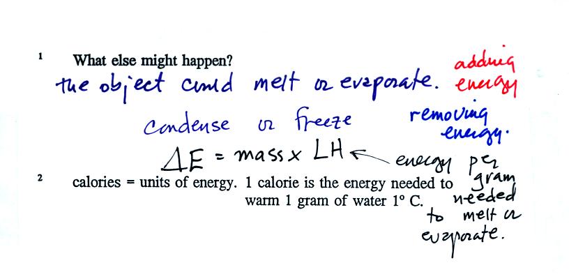
The equation above tells you how much energy must be added
to cause a
material to melt or evaporate (or how much energy must be removed to
cause the material to condense or freeze). LH stands for "latent
heat."
A small
experiment was performed at the end of class to make use of these two
equations (the equation relating energy and temperature change and the
latent heat equation just mentioned). The goal of the experiment
was to measure the latent heat of vaporization of liquid nitrogen - the
energy needed, per gram, to evaporate nitrogen.
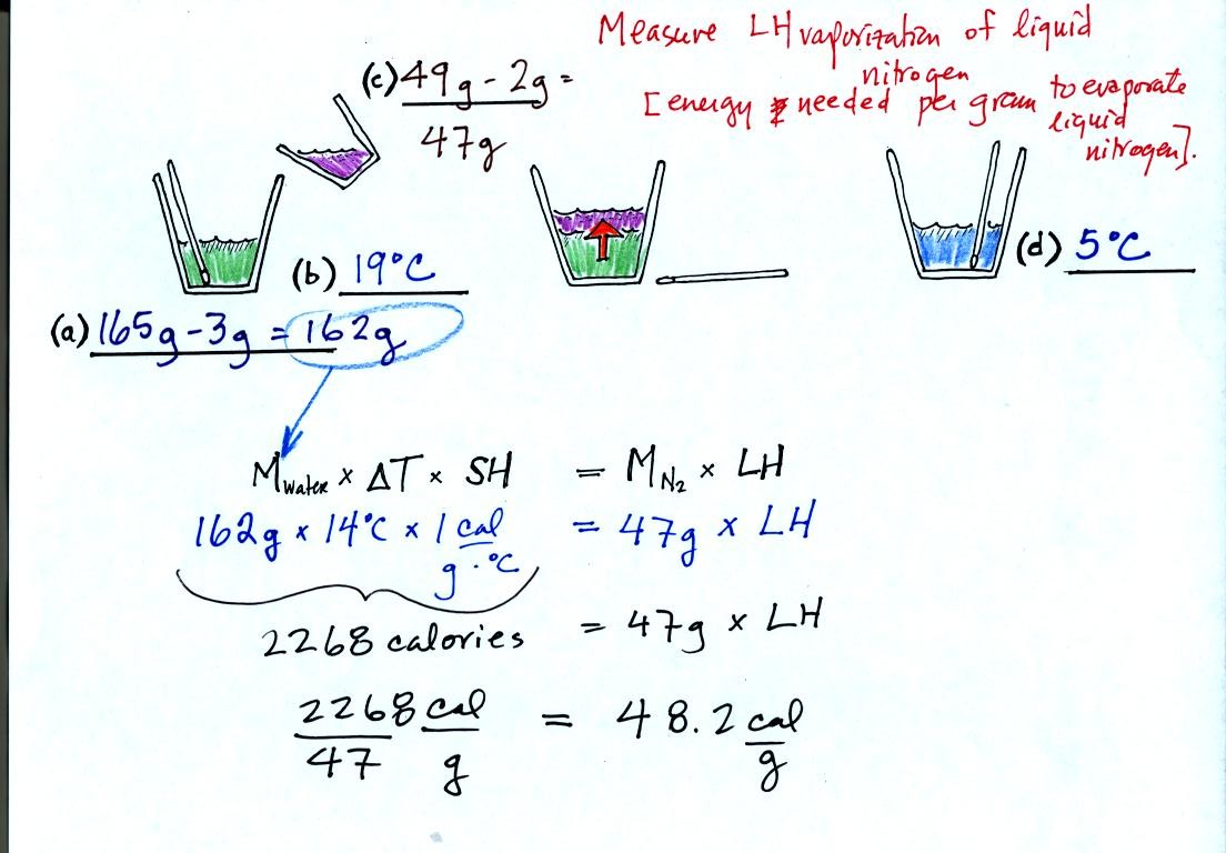
We first measure the mass and temperature of some
water [(a) and (b) above]. The water plus the cup weighed 163
g. We subtracted
the 3 gram weight of the cup.
The
water will be the source of the energy needed to evaporate liquid
nitrogen. By measuring the temperature of the water before and
after the liquid nitrogen is evaporated, we will be able to determine
how much energy was used.
We also need to measure the mass of liquid nitrogen (the cup
weighed 2 g) [step (c)].
We don't
need to worry about the temperature, it's -320 F. The liquid
nitrogen can't get any warmer than that and still remain a liquid.
We pour the liquid nitrogen into the cup of water and
wait (middle picture).
Energy will flow from the warmer water into the very much colder liquid
nitrogen. We perform the experiment in a styrofoam cup and assume
that no energy is flowing into the air in the room (because the water
started out at room temperature there won't be much energy flowing from
the water into the room anyway).
Now we remeasure the temperature of the water. The
water should
be colder because some of its energy was used to evaporate the
nitrogen. We assume that the mass of the water has stayed the
same.
Now we use an energy balance equation. On the left is
the energy
taken from the water. Removing this energy cooled the water from
19 C to 5 C, a change of 14 C. The specific heat of water is 1
calorie per gram per degree Celsius. On the right is the energy
needed to evaporate the liquid nitrogen. In our case we
evaporated 47 grams. We plug in all our measurements and solve
for LH.
We obtained 48.2 calories per gram. The known value is 48
cal/g. So our measurment was very close (the experiment didn't
work as well in the Wed. class - the measured value was 57.5
cal/g).