Tuesday Apr. 19, 2011
click here to
download today's notes in a more printer friendly format
Homework #6 was returned today together with a set of
solutions. That will probably be the last homework assignment of
the semester.
Today we will be looking at satellite detection and location of optical
emissions produced by lightning. In order to reduce the
background signal from reflected sunlight the sensors isolate just a
single bright emission in the lightning spectrum. So this seems
like a good place to mention lightning spectroscopy and show you an
example of the
optical spectrum of lightning. We'll come back to this topic on
Thursday and how spectra can be used to estimate lightning channel
temperatures.
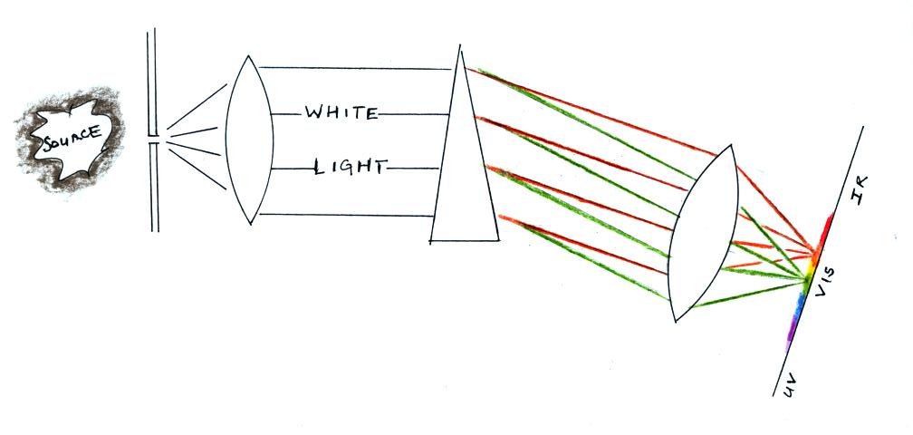
The figure below shows a conventional spectrometer or
spectrograph. The front of the spectrometer is pointed at a light
source. Light from the source first passes
through a narrow slit (the width of the slit will partly determine the
wavelength resolution of the spectrometer, i.e. whether it will be
possible to separate closely spaced emission features in the
spectrum). Rays emerging from the slit are collimated by a lens
and then passed through a prism (or a diffraction grating). The
light is refracted (bent) and dispersed (split into colors; the amount
of bending depends
on the wavelength). A second
lens focuses the parallel rays of light onto a detector or a piece of
film.
You can eliminate the slit in the case of lightning because the
lightning channel itself is narrow. Lightning spectrometers also
often use both a prism and a diffraction grating. This has the
effect of "straightening out" the spectrometer so that it is easier to
point at lightning. The diffraction grating might also increase
the dispersion.
An example of an actual spectrum is shown below (source: Lightning
Spectroscopy,
E.P.
Krider,
Nuclear Instruments and Methods, 110,
411-419, 1973 (link to a PDF file) )

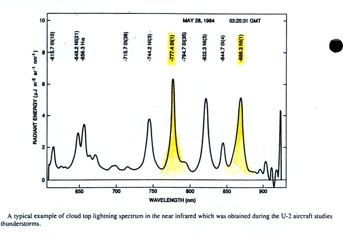
This spectrum extends from the
near-ultraviolet to the near-infrared. The first line in the Balmer Series
for hydrogen (Halpha at 6563
Angstroms) can be seen clearly (the
hydrogen comes from the dissociation of water vapor by the
lightning). Note also the bright lines at 7774 and 8683
Angstroms. These are emissions from atomoic oxygen and nitrogen
respectively (OI and NI denote atomic oxygen and nitrogen). The
OI line at 7774 is used by the satellite detectors that we will be
discussing.
The satellite sensors that we will be discussing were designed by
researchers at the NASA Marshall Space Flight Center in Huntsville
Alabama. An initial step in their program was to make
measurements of lightning optical emissions from high-altitude aircraft
flying well above the tops of the thunderclouds (a U-2 aircraft flying
at appoximately 20 km altitude). A publication "The
Detection
of
Lightning From Geostationary Orbit," summarizes
results from the aircraft measurements and discusses some of the
factors that must be considered in the design of a satellite lightning
sensor.
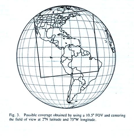
The area viewed by a lightning mapper aboard a satellite in
geostationary orbit. We will learn that most lightning activity
falls between 35 S and 35 N latitude.
Lightning near-IR emissions measured above cloud top from a
high-altitude airplane. The 777.4 nm and 886.3 nm features (OI
and NI) each contain 5 to 10% of the optical energy in a lightning
flash. The 777.4 nm line was chosen for the satellite detector.
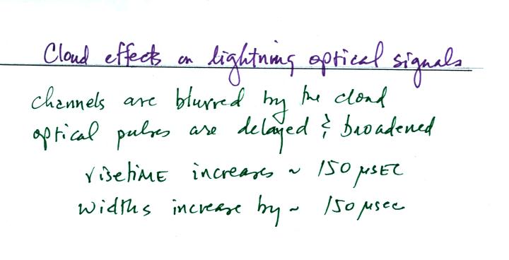
Just like frosted glass, clouds will blur any image of the
lightning channel inside the cloud. The optical signal risetime
and pulse width are each increased by about 150 microseconds. The
following figure helps to understand why this is true.
Photons
emitted by a lightning channel are scattered (redirected) multiple
times before leaving the cloud. The path in pink undergoes a
relatively low number of scatters. The green path is scattered
more times and takes longer to escape from the cloud. It is
difficult to distinquish between cloud-to-ground and intracloud
discharges.
Somewhat surprisingly perhaps, there is very little absorption of
the light signal by the cloud.
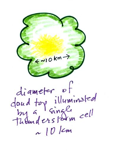
A lightning flash illuminates about 10 km diameter of the cloud
top (sorry I do get carried away with the colored pencils).
Ideally this would fill a pixel on the CCD satellite detector.
We spent most of the remainder of the class discussing the Optical
Transient Detector OTD). This is the first of two satellite
"lightning mappers" designed by the people at the NASA Marshall Space
Flight Center. You can read more about that research group and
some of the activities on the Global Hydrology and
Climate Center webpage.
The OTD was a prototype for the Lightning Imaging Sensor.
The OTD was launched on Apr. 3, 1995 and turned off in Mar. 2000,
having operated 2 years beyond its expected lifetime.
It was launched into a nearly circular orbit 740 km (~450 miles)
high. The orbit was inclined 70o
(relative to the Equator) so the
satellite coverage extended from 75o
S to 75o N latitude.
The field of view was about 1300 km x 1300 km (about 1/300 th of
the earth's surface) and was imaged onto a 128 pixel x 128 pixel CCD
sensor array (thus about 10 km x 10 km per pixel which is about the
size of the cloud top illuminated by lightning)
Location accuracy (at nadir) was about 8 km.
The orbit precesses about 15 minutes (1/4 of a degree) per day.
It takes about 50 days for the satellite to review a specific location
on the earth's surface at the same time of day.
In a year the OTD images most locations for a total time of > 14
hours (400 individual over passes).
The OTD detects lightning during the day and at night. The
typical daylight cloud background (sunlight reflected off the cloud
tops) is 50 to 100 time brighter than lightning.
Several steps must be taken in order to detect lightning signals
superimposed on this bright background.
(i) The pixel size corresponds roughly to the size of the
cloud top illuminated by lightning.
(ii) A 1 nm narrow band interference filter centered on the 777.4
nm OI emission was used. Much of the cloud
background
falls at other wavelengths and was
blocked.
(iii) CCD signals were integrated for 2 ms - well over the duration of
the lightning optical pulse.
(iv) successive frames were subtracted. This subtracts out much
of the slowly time varying background signal
This last process is illustrated below
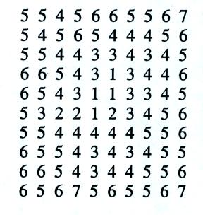
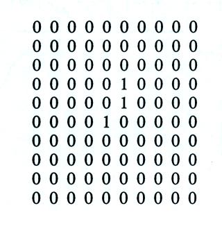
The leftmost image shows a picture of the scene. The middle two
frames show the CCD data for pictures taken of the scene with and
without a lightning. It's hard to see the lightning until you
difference these middle images. The lightning appears in the 4th
picture (the three pixels with values of 1 in the middle of the scene).
There are still sources of noise such as sun glint that create
erroneous lightning counts. The South Atlantic Anamoly is also a
source of false triggers. This is a region where the Van Allen
Radiation Belts make their closest approach to the earth's
surface. The inner belt contains mainly high energy
protons. When the satellite passes through the belt, the high
energy particles strike the CCD array and produce anamolous triggers.
We looked at some images of lightning activity derived from OTD
data.
Here's the first image showing all of the lightning detected in
1999.
Most of the lightning detected is found over land affected by the
Intertropical Convergence Zone (ITCZ). This refers to a feature
in the 3-cell model of the earth's global scale circulation pattern.
The ITCZ is nominally located near the Equator (also labelled the
equatorial low in the figure above). It will move north of the
Equator in summer (northern hemisphere summer) and south of the equator
in the winter. You can usually see a band of clouds on global
satellites
photographs that are associated with the ITCZ.
Here's the lightning detected during the months of December, January,
and February 1999. Note how the activity has shifted into the
southern hemisphere. The activity at higher latitudes in the
northern hemisphere might be associated with storms forming along the
polar front.
This is the June, July and August map for the same year. Activity
is now primarily in the northerm hemisphere.
78% of the lightning detected (and remember the OTD doesn't distinguish
between cloud-to-ground and intracloud discharges) is found between 30
S and 30 N latitude. 88% of the lightning is found over
continents, islands, and coastal regions. There is much less
activity over the oceans.
Here is a link to the source
of
these
OTD
GIF
Images
One interesting result from 5 years of OTD lightning data is a new
estimate for the global lightning flashing frequency:
44
+/-
5 flashes/sec
This is about half of the 100
flashes/sec value that was long thought to be true. The 100
flashes/sec value dates back to 1925.
We were starting to run short of time so we finished with just a quick
mention of the Lightning Imaging Sensor launched on Nov. 28, 1997 into
an orbit with 35 degree inclination. The LIS mapper is still
operating. You can read more about its design and look at
examples of data here.