Tue., Jan. 22 - Review of electrostatics pt. 2

We'll insert this into the expression for electric field.

It is often much simpler to determine the electrostatic potential because it is a scalar quantity. The electric field can then be determined by taking the gradient of the potential.

The expression above is valid for a point charge. More general expressions for cases where multiple charges are present or when charge is distributed over a volume or on a surface are shown below. This figure wasn't drawn in class.

Essentially you can break a more complex charge distribution into smaller pieces and then either sum over a collection of multiple discrete charges, or integrate over volume or surface distributions of charge to determine the electrostatic potential.

When the curl of a vector field is zero the vector field is irrotational. I showed an online animation showing both irrotational and rotational vortices.

The pattern of electric field vectors around a positive charge would look something like this. If we were to place something in the field (as was done in the animation above) and watch it move it would move outward without any rotation.

An irrotational field has another important property. A line integral from r1 to r2 will be independent of the integration path. I didn't mention this in class.

Because the curl is zero we can used Stokes' Theorem to say the line integral of the vector around a closed loop is also zero. The rest of the argument follows fairly simply from that.

We might sometimes have occasion to perform a line integral of electric field.

There may be situations where E is known. We can determine the potential as shown above.

Let's assume a point charge and substitute in an expression for E into the left integral above.

We'll set this equal to the earlier expression

We get our earlier result (provided we assume that Φ(r = ∞) is zero)

We can write the electric field as the gradient of the electrostatic potential and then substitute that into Gauss' Law.

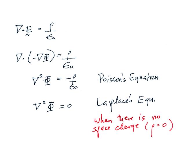
We obtain Poisson's Equation. Laplace's equation applies in situtations where the volume space charge density is zero. We'll be using Laplace's equation in our next lecture. Here is a handout with vector differential operators (Laplacian, curl, gradient and divergence) in cartesian, cylindrical, and spherical coordinate systems.

Now some applications of what we have been learning. In this and the next class we'll looking at a couple of instruments used to measure thunderstorm and lightning electric fields.

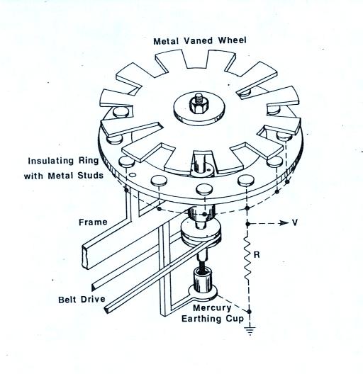
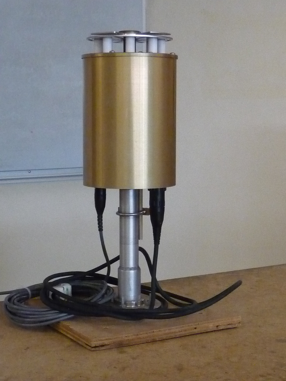
The first is an electric field mill used to measure static and slowly time varying electric fields. Referring to the figure below at left (from Uman's 1987 The Lightning Discharge book). The sensors (referred to as studs in the figure) are covered by a rotating grounded plate. 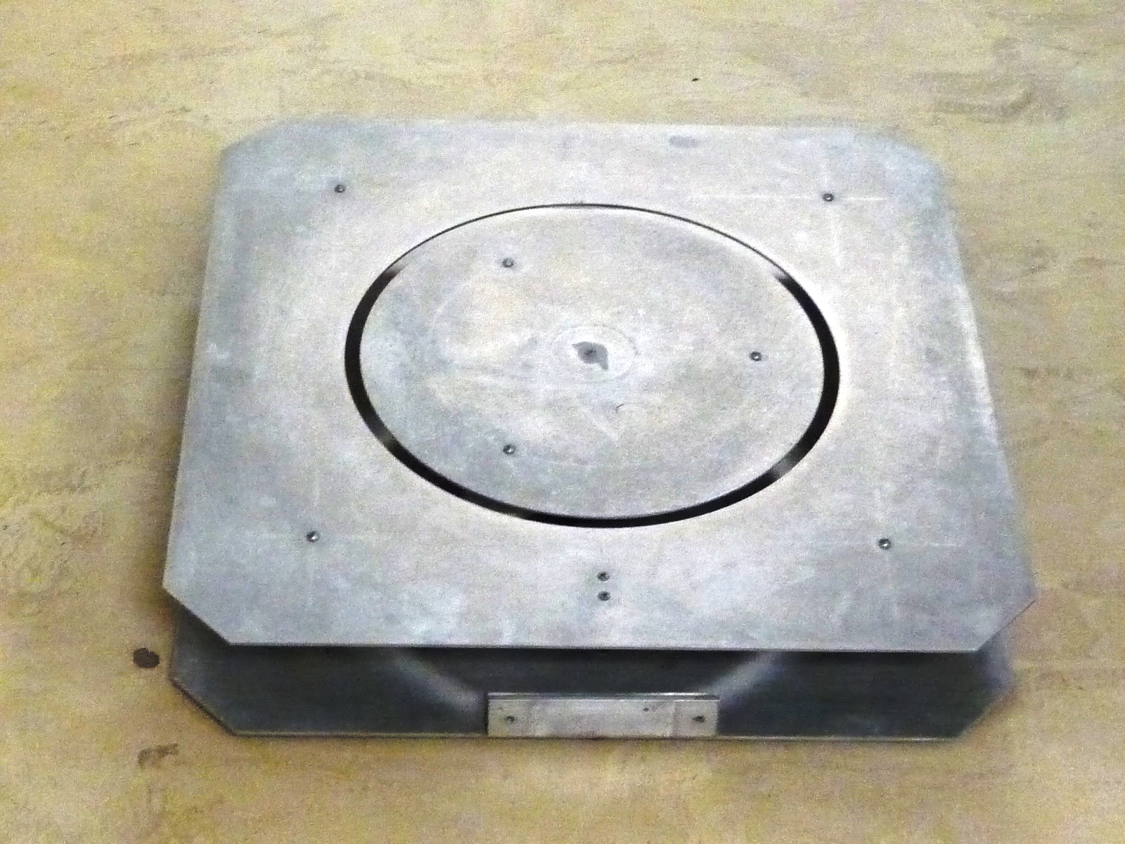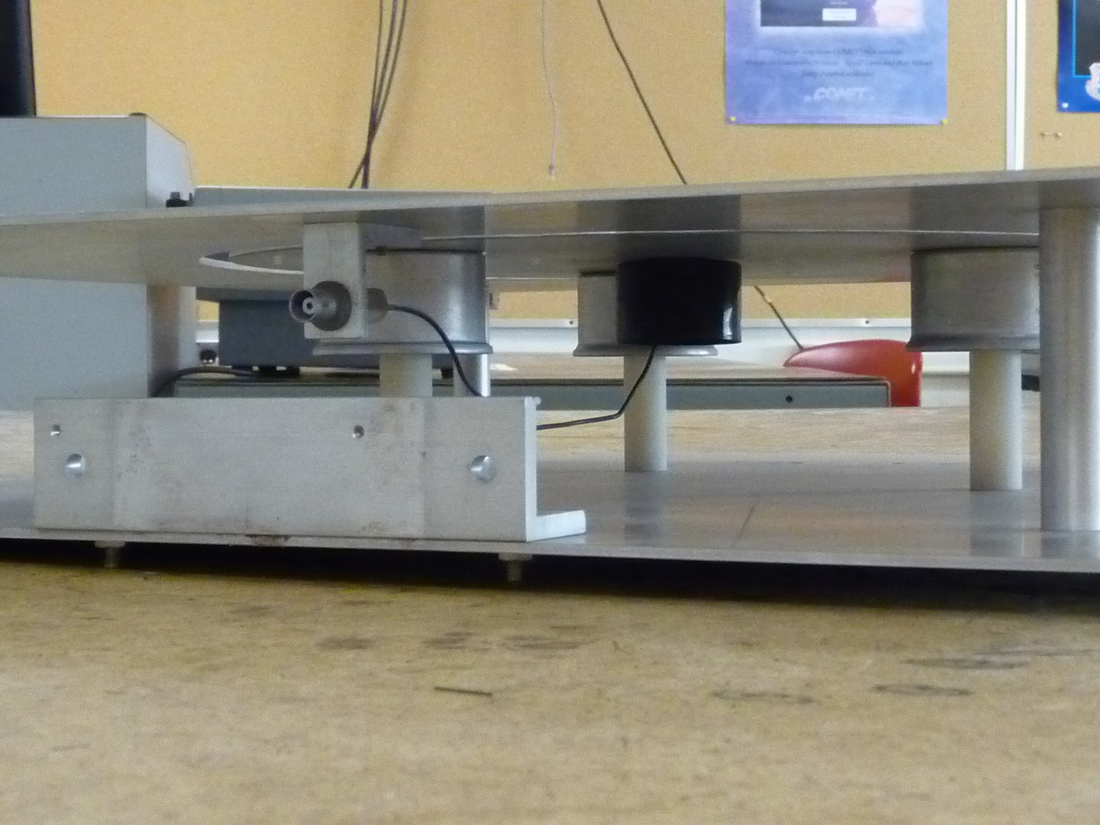The rotating plate is notched or slotted so that the sensors are periodically exposed to and covered (shielded) from the ambient electric field. A photograph of the field mill shown in class is shown below at right (signal and power cables are connected at the bottom of the mill).

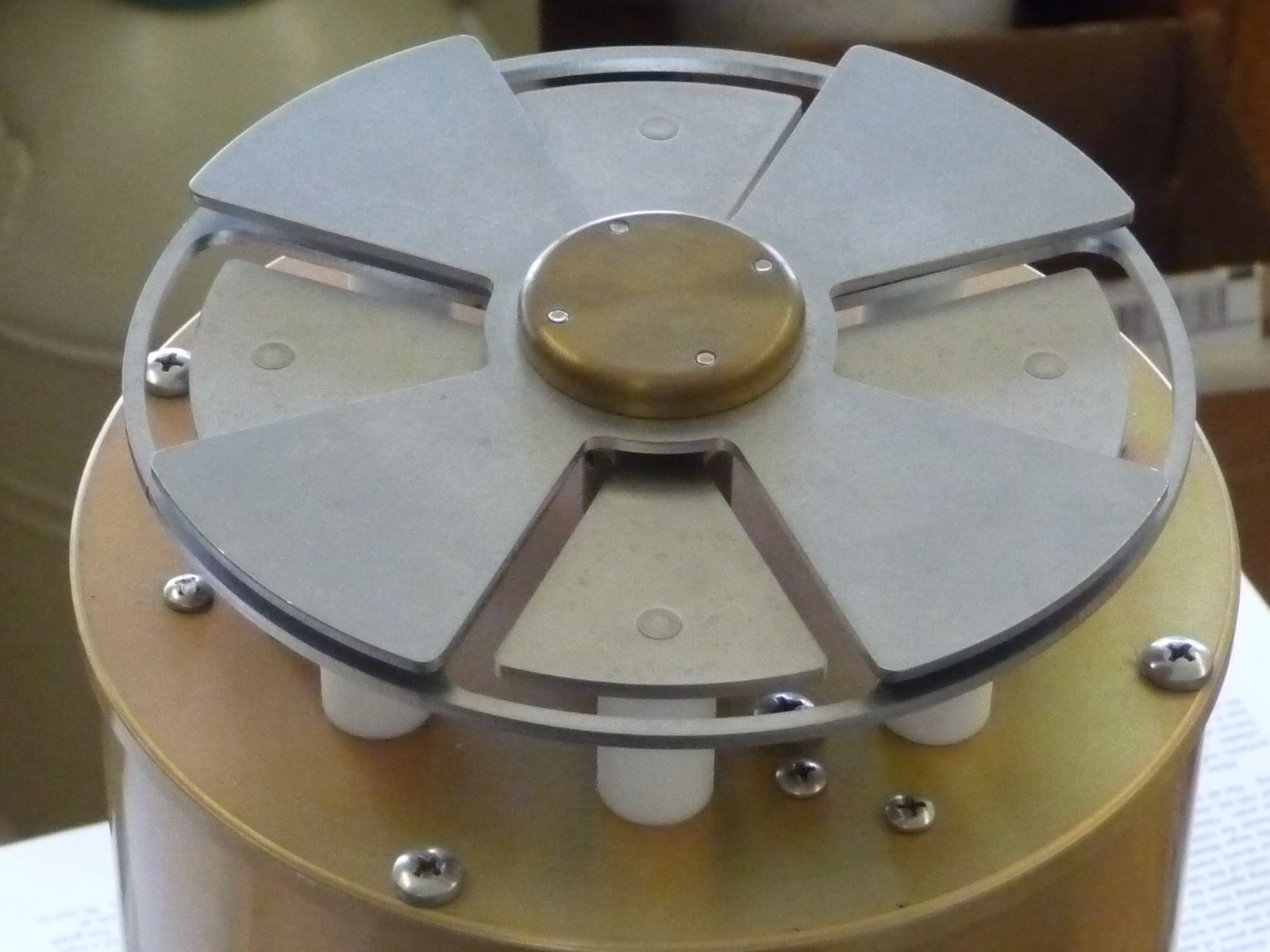
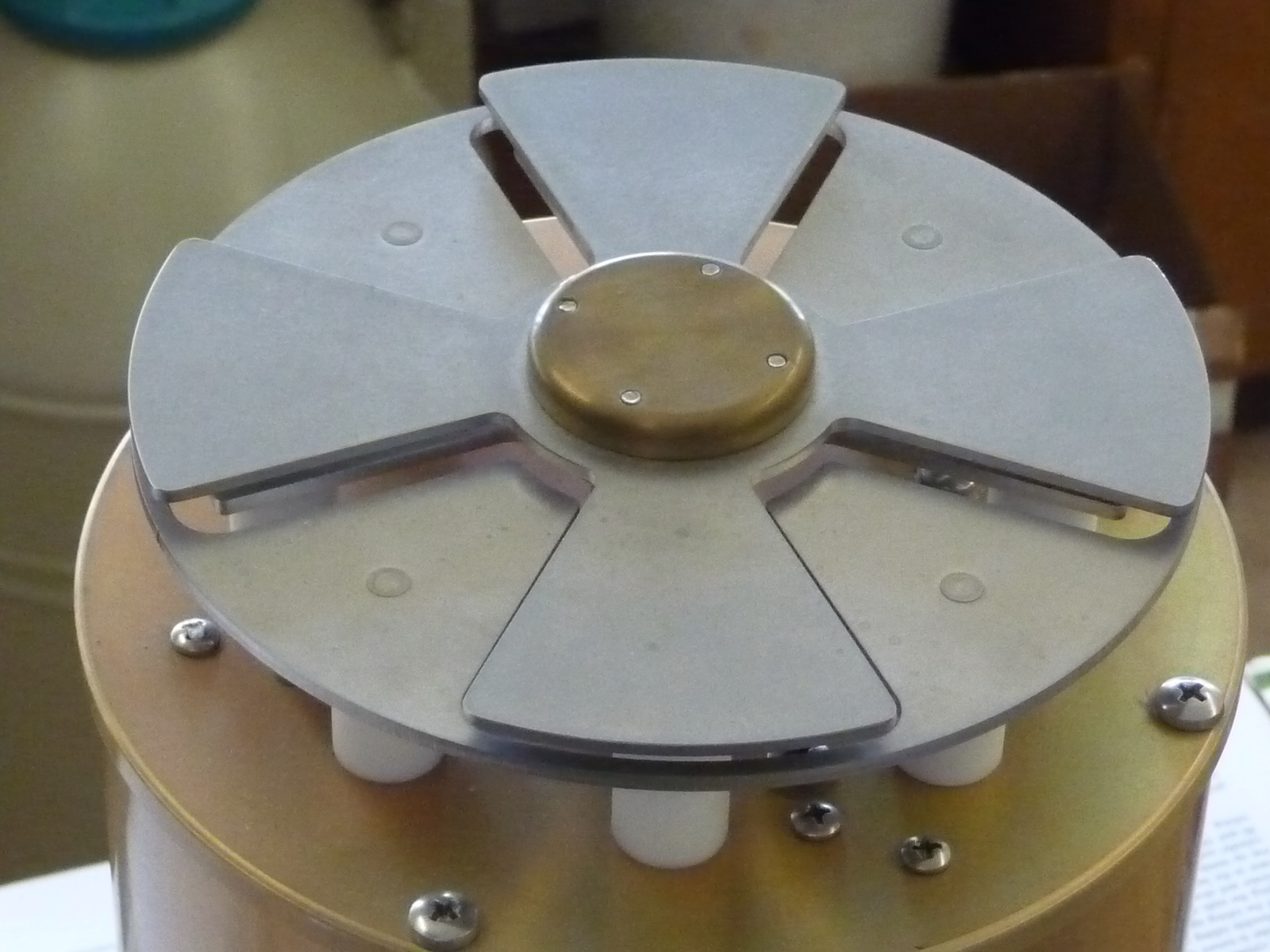
The two photographs below are closeups of the top of the field mill

The stator plates are exposed to the E field at left and covered in the photograph at right. The four stators (sensor plates) exposed in the figure at left are connected together electrically. Another four stators, also connected together are exposed in the figure at right. Thus this field mill has two sets of sensors. One is exposed while the other set is covered. This just makes it possible to make measurements of the E field two times more often.

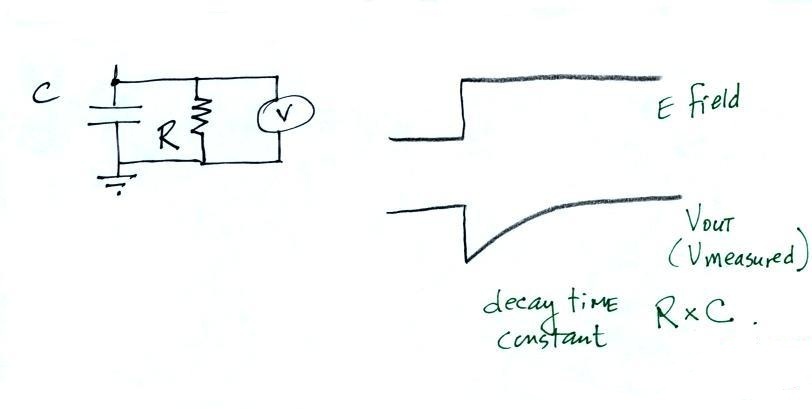
The next figure shows currents flowing into and out of the sensor plate in response to an incident E field.

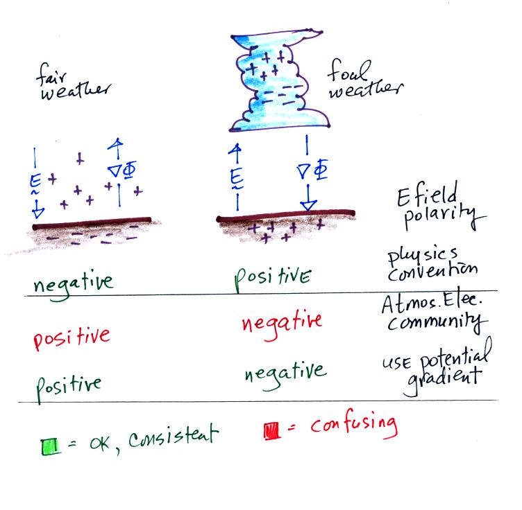
The sensor plate is covered at Point 1. At Point 2 the sensor is uncovered and we assume the ambient field points upward (toward negative charge in the lower part of a thunderstorm perhaps). Positive charge flows up to the sensor plate. The current flows from the sensor in Point 3 because the sensor has been covered and shielded from the E field. Points 4 and 5 are similar except the polarity of the E field has been changed.

Note the current signals at Points 2 & 5 are the same even though the field polarities are reversed. You must keep track of when the sensor is covered and uncovered in order to determine the polarity of the incident E field.

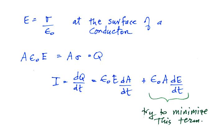
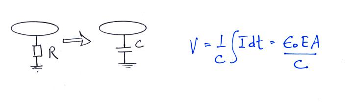
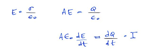
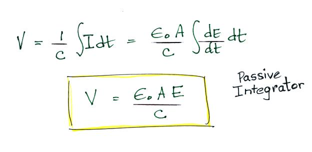
It is a relatively simple matter to relate the amplitude of the signal current to the intensity of the incident E field.

We use the expression derived a few days ago relating the E field at the surface of a conductor and the surface charge density (sigma in the equations above). A is the area of the sensor.

If you integrate the current (connect the sensor through a capacitor to ground) you obtain an output voltage that is proportional to E.

We were able to separate charge and electrify a couple of objects using triboelectric charging (see the handout from class on Tue., Jan. 15). For example rubbing a rubber (or perhaps latex) balloon with cat or rabbit's fur should charge the balloon negatively. We were able to verify when the charged balloon was held above the field mill and we saw a negative polairty output signal. The same thing happened when PVC pipe was used. Rubbing a glass graduated cylinder with fur charged the glass positively.

We were also able to confirm that the dome on the Van de Graaff generator was indeed negatively charged as mentioned in last Tuesday's class.

Next we looked at an example of an E field record obtained with an electric field mill. The data come from the Kennedy Space Center field mill network.

The first record is interesting because it shows the transition from fair to foul or stormy weather electric fields (a change in polarity and in field strength).

At the very beginning of the record fields are about 200 V/m. The field crosses zero at about 20:39:00 GMT and increases in amplitude, eventually reaching about -2500 V/m. The abrupt transitions are caused by lightning. In our next lecture we will expand the time scale and look at the field variations that occur in an individual discharge. Later in the course we'll come back to field records like this and show what we start to learn something about the locations of charge and amounts of charge involved in lightning discharges by analyzing these electric field changes.

Note that the vertical axis is labeled potential gradient rather than electric field. This brings up a confusing situation regarding electric field polarities that you should be aware of; something that might cause some confusion if you ever read through some of the atmospheric electricity literature.

The figure above at left correctly show the E field pointing downward toward negative charge on the earth's surface during fair weather. The E field reverses direction under a thunderstorm. The main negative charge center in the cloud causes positive charge to build up in the ground under the storm. The E field points upward.

A physicist would consider the fair weather field to be negative polarity because it points downward and would call the stormy weather field positive. The atmospheric electricity community will often refer to the fair weather field as positive and would call the foul weather field negative. This is a source of confusion.

Nowadays atmospheric electricians either just simply use the physics convention or refer to the potential gradient rather than the electric field. In fair weather a negative E field (physics convention) and a positive potential gradient are consistent.

Later in the course we will find that lightning discharges consist of a sequence of discharge processes. Because a lightning discharge only last 1 second or so it appears as just an abrupt field change on the record above. Some lightning processes occur on millisecond, microsecond and even sub microsecond time scales. The figure below illustrates this (don't worry about all the details and names at this point, we'll come back to this later in the semester). An electric field mill can measure static and slowly varying fields but can't resolve all the field changes and variations that occur on faster time scales.

One way of measuring these faster time varying electric fields is to use a flat plate antenna (aka flush plate dipole antenna). It basically consists of a large flat grounded plate that would be positioned on the ground (preferably flush with the surrounding ground). A smaller circular insulated sensor plate is found inside a center hole as shown in the photograph below (the antenna is on the classroom floor in this photograph).

We look under the top plate of the antenna in the next picture.

The center sensor plate is supported by insulating nylon or teflon spacers. The top end of the supports are covered with "rain hats" to try to keep the insulators dry during rainy weather. A wire connection to the center plate connects to a BNC cable to carry the signal to processing and recording equipment.

In some ways the operation of this antenna is similar to the field mill. In this case a time varying E field causes current to flow to and from the center sensor plate (you don't need to repeatedly cover and uncover the sensor plate).

This current is proportional to the time derivative of the electric field (σ in the equation below is the surface charge density on the sensor plate).

Integrating the current gives an output signal that is proportional to E.

In the circuit above the antenna is connected to a capacitor, this is a passive integrator. Some kind of measuring device would then be connected across the capacitor.

In some cases the input impedance of the measuring device together with the capacitance in the passive integrator (a small capacitance would provide higher gain) gives a time decay constant that is too short (the time constant should be several times larger than the field variations that you are measuring). In this case an "active integrator" circuit is needed. We'll look at this in class on Thursday.