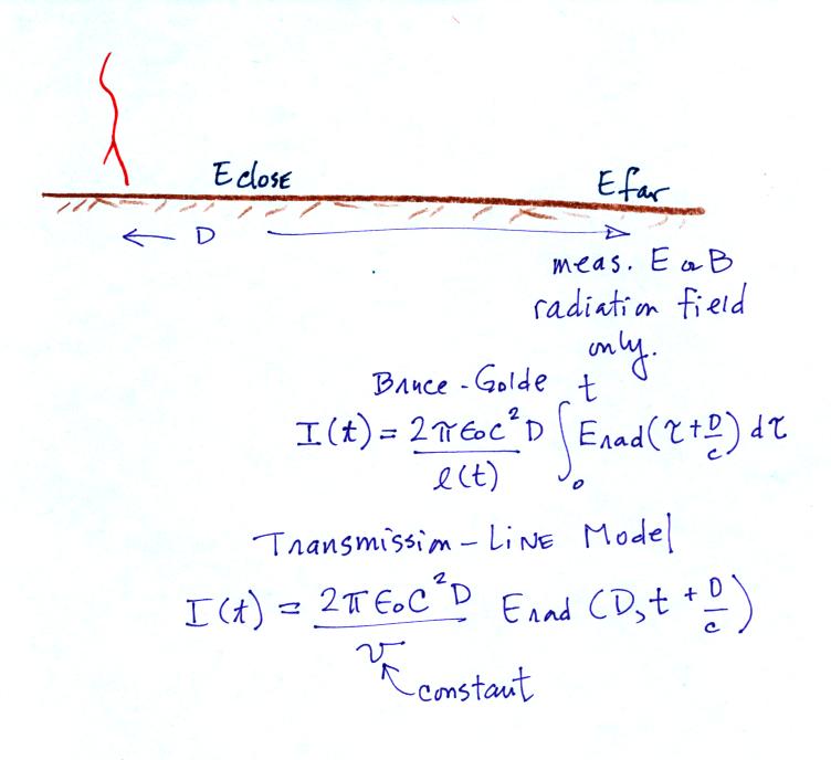
Here is one of the ways that the
Bruce-Golde (BG) and the transmission line (TL) models were tested
experimentally. Measurements of electric and magnetic fields were
measured at 2 stations: one close to and the other far from the strike
point. The far field measurements (which are just radiation
fields
and don't contain any induction or electrostatic fields) were used to
determine the return stroke channel current, I(t), using the two
equations above. Then both near and far fields were calculated
and compared with the
actual measurements at the two sites.
Here are some of the results from the tests.
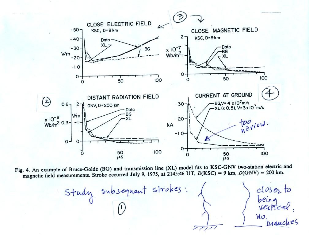
The experimental tests used only the fields from subsequent strokes (1) because, without branches, they are closer to the model assumptions that the lightning channel is straight and vertical. A constant return stroke propagation speed was assumed and was adjusted to give the best fit between measured and computed fields.
At (2) the distant measured radiation field is used to derive the Bruce Golde (BG) and Transmission Line (TL) model return stroke current I(z,t). Then the E radiation fields are computed using both the BG and TL currents. You can see for the distant fields, the agreement is pretty good.
The agreement isn't quite as good for the close fields (3).
The derived channel currents are shown in (4). The TL current waveform is too narrow and is unrealistic.
Here are some of the results from the tests.
The experimental tests used only the fields from subsequent strokes (1) because, without branches, they are closer to the model assumptions that the lightning channel is straight and vertical. A constant return stroke propagation speed was assumed and was adjusted to give the best fit between measured and computed fields.
At (2) the distant measured radiation field is used to derive the Bruce Golde (BG) and Transmission Line (TL) model return stroke current I(z,t). Then the E radiation fields are computed using both the BG and TL currents. You can see for the distant fields, the agreement is pretty good.
The agreement isn't quite as good for the close fields (3).
The derived channel currents are shown in (4). The TL current waveform is too narrow and is unrealistic.
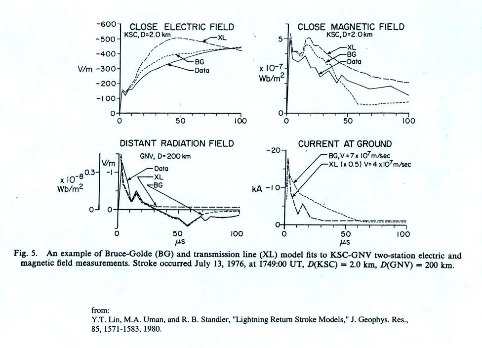
An additional set of test results.

A return stroke velocity was assumed for each set of near and far
E and B field measurements (the velocity value was adjusted to give the
best fit between measured and calculated fields). The velocity
values derived for the BG model are shown in the top graph and appear
to be distance dependent (distance from the close station to the
lightning strike point). That is a physically unreasonable
result. The velocities derived for the TL model appear in the
bottom plot. The values are reasonable and do not appear to vary
with distance.
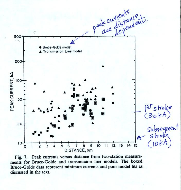
Here are the peak current values derived for both the TL and BG models. In both cases peak current values appear to be distance dependent which is not realistic. Many of the TL peak currents are too large. First return stroke peak currents are typically about 30 kA. Subsequent stroke peak currents are usually less. Some of the TL peak currents in the plot above exceed 100 kA.
Despite its deficiencies, the TL model is still widely used to infer peak current and peak current derivative values from measurements of electric and magnetic radiation fields. We'll next discuss probably the best and most complete test of the TL model.
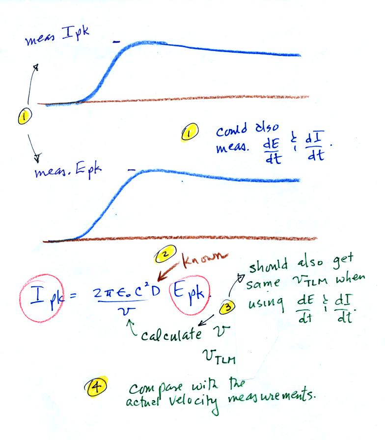
Here's the basic idea. The experiment used rocket triggered
lightning, so the return stroke current could be measured
directly. The electric radiation field is measured at one or more
sites. The current and field derivatives (dI/dt & dE/dt) were
also be measured.
Then you stick the measured Ipk and Epk values into the transmission line model equation and solve for the velocity (the field measurements are made at known distance from the triggering site). You should get the same velocity value if you used dI/dt and dE/dt in the TL model equation.
Then you compare the computed velocity with a direct measurement of velocity made with a high speed streaking camera.
Here are the peak current values derived for both the TL and BG models. In both cases peak current values appear to be distance dependent which is not realistic. Many of the TL peak currents are too large. First return stroke peak currents are typically about 30 kA. Subsequent stroke peak currents are usually less. Some of the TL peak currents in the plot above exceed 100 kA.
Despite its deficiencies, the TL model is still widely used to infer peak current and peak current derivative values from measurements of electric and magnetic radiation fields. We'll next discuss probably the best and most complete test of the TL model.
Then you stick the measured Ipk and Epk values into the transmission line model equation and solve for the velocity (the field measurements are made at known distance from the triggering site). You should get the same velocity value if you used dI/dt and dE/dt in the TL model equation.
Then you compare the computed velocity with a direct measurement of velocity made with a high speed streaking camera.
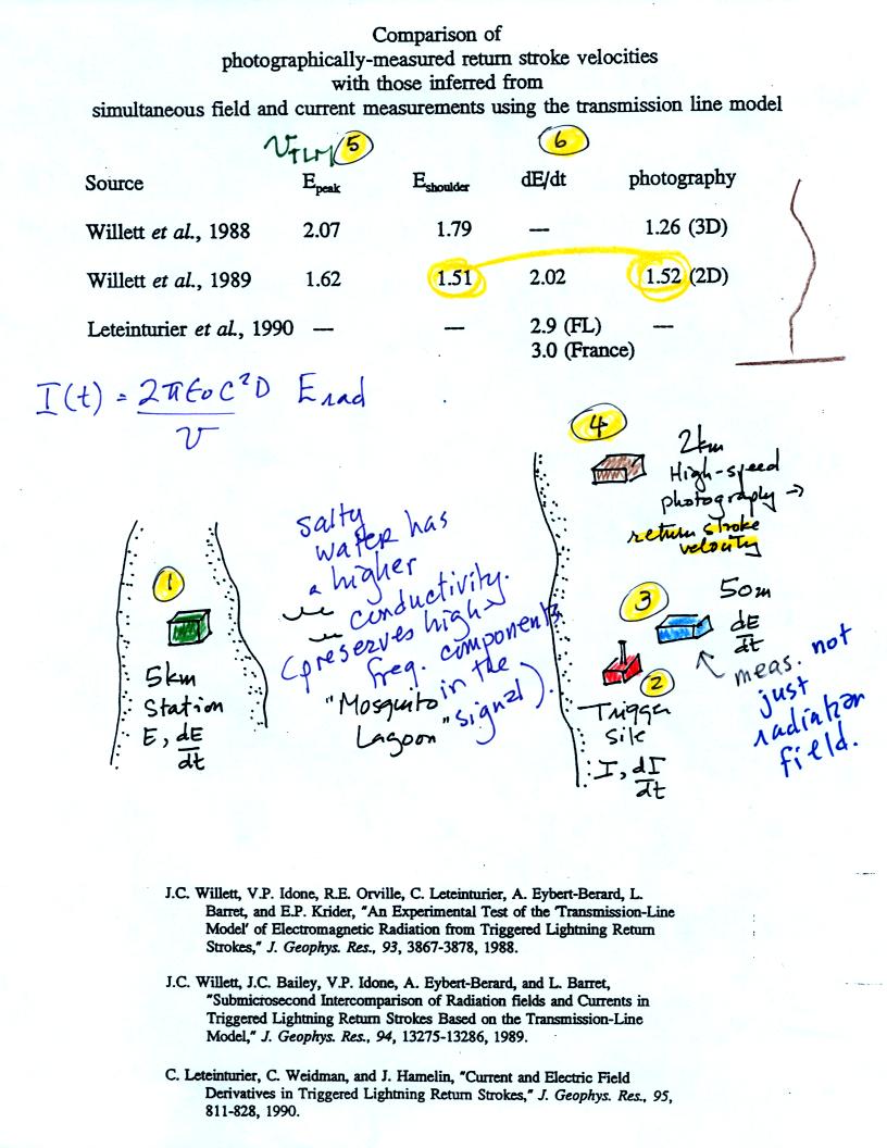
Here's the layout of the
experiment. It was conducted at the Kennedy Space Center (near a
place called "Mosquito Lagoon")
Lightning was triggered at Point 2 in the figure, that's where I and dI/dt were measured. dE/dt was measured at Point 3, just 50 m from the trigger point. That is probably too close. The measured fields probably had induction and electrostatic field contributions.
Return stroke velocity was measured at Point 4.
E and dE/dt were measured at Point 1, 5 km from the triggering point. Propagation between Points 1 and 2 was over salty water so the high frequency content of the electric fields would be preserved.
Point 5 shows the velocity values computed using E fields. The experiment was conducted in two successive years (1985 and 1986 if I remember correctly). The two velocity values 2.07 and 1.62 (x 108 m/s) should be compared with measured values of 1.26 and 1.52 (x 108 m/s). A "cleaner" triggering setup was used in the second year, that may explain the better agreement between calculated and measured velocities (1.62 and 1.52).
Better agreement between measured and computed velocities is obtained using E shoulder values rather than E peak values. We'll explain what that refers to in a minute. Note also that the velocity values derived using dE/dt are different from those derived from E.
The TL model would predict that the current and electric field waveforms would have identical shapes. In reality the E field waveforms have some addtional structure that is not on the current waveforms. This is illustrated below.
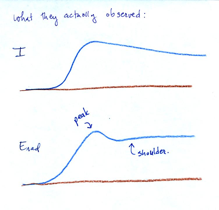
The E field waveform has a small peak that is followed by a
shoulder.
We can reproduce this feature if we assume that the return stroke begins with two current waves propagating upward and downward from a point above the ground (the point where the stepped leader and upward connecting discharge meet).
Lightning was triggered at Point 2 in the figure, that's where I and dI/dt were measured. dE/dt was measured at Point 3, just 50 m from the trigger point. That is probably too close. The measured fields probably had induction and electrostatic field contributions.
Return stroke velocity was measured at Point 4.
E and dE/dt were measured at Point 1, 5 km from the triggering point. Propagation between Points 1 and 2 was over salty water so the high frequency content of the electric fields would be preserved.
Point 5 shows the velocity values computed using E fields. The experiment was conducted in two successive years (1985 and 1986 if I remember correctly). The two velocity values 2.07 and 1.62 (x 108 m/s) should be compared with measured values of 1.26 and 1.52 (x 108 m/s). A "cleaner" triggering setup was used in the second year, that may explain the better agreement between calculated and measured velocities (1.62 and 1.52).
Better agreement between measured and computed velocities is obtained using E shoulder values rather than E peak values. We'll explain what that refers to in a minute. Note also that the velocity values derived using dE/dt are different from those derived from E.
The TL model would predict that the current and electric field waveforms would have identical shapes. In reality the E field waveforms have some addtional structure that is not on the current waveforms. This is illustrated below.
We can reproduce this feature if we assume that the return stroke begins with two current waves propagating upward and downward from a point above the ground (the point where the stepped leader and upward connecting discharge meet).
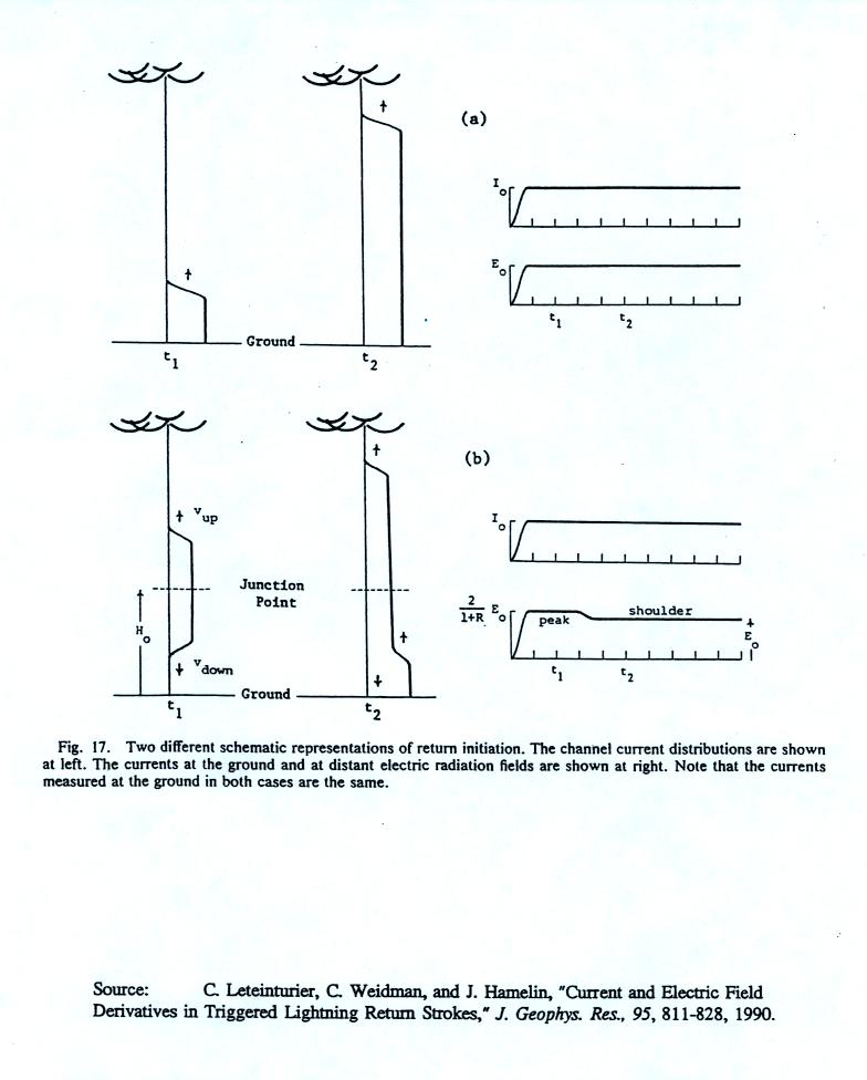
This figure compares the E field
waveforms produced by (top) a single current wave propagating upward
from the ground and (bottom) two waves propagating upward and downward
from a junction point above the ground.
Now here's a quick and probably somewhat confusing explanation of how the two wave model can produce a peak and a shoulder in the E field waveform.
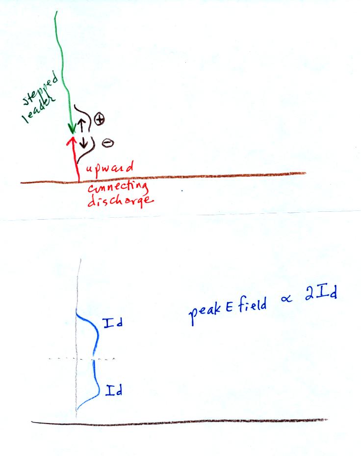
Waves each with a peak current of Id move upward and downward from
the junction point (positive polarity moving upward, negative polarity
moving downward). We assume that the current reaches a peak
before the downward moving wave reaches the ground. Each of these
waves will contribute to the electric field. The peak E field
value will be proportional to 2 x Id.
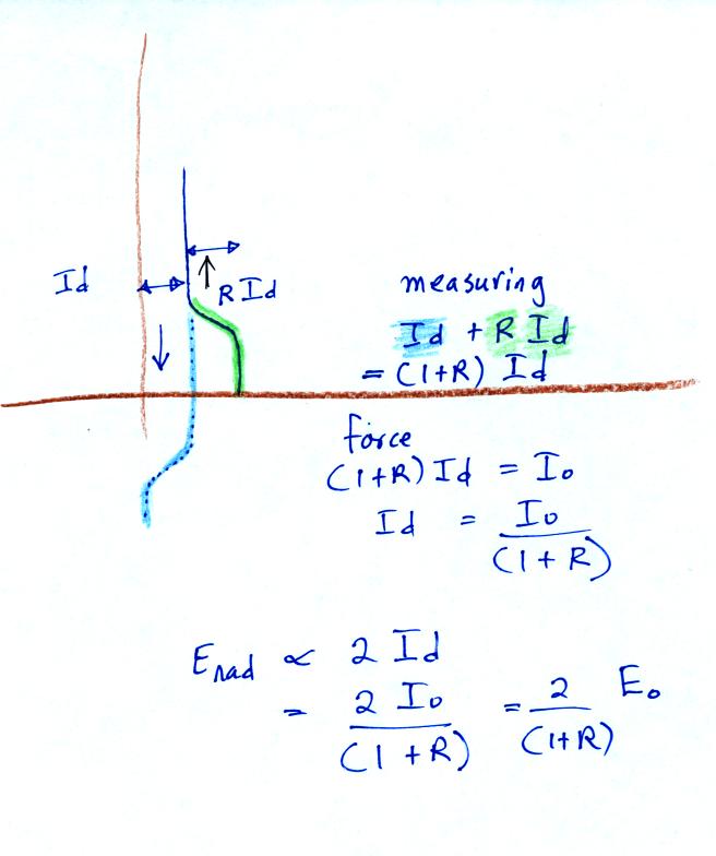
The downward wave reaches the ground, a portion R x Id is
reflected upward. So what is measured at the ground is Id + R x
Id = (1 + R) Id. We force this to be equal to Io, the amplitude
of a single current wave moving upward from the ground. The two
current waveforms measured at the ground would be
indistinquishable. This explains how you arrive at an E field
peak value of 2 Eo / ( 1+R ) .
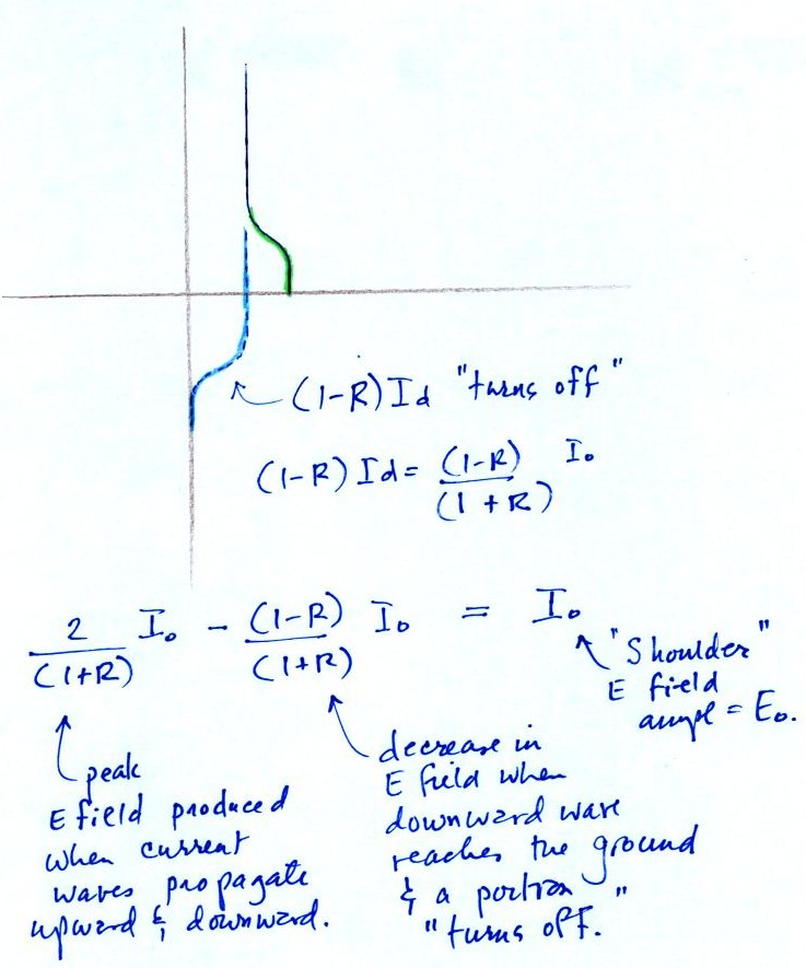
A portion of the downward current wave (the part that isn't
reflected) turns off. This will cause a decrease in the E
field. So we take the peak E field value [ 2 Eo / (1 + R) ] and
subtract the decrease caused by the turn off. You end up with a
shoulder E field value of Eo.
We ended the day with a look at some experimental measurements of distant electric radiation fields and estimates of peak I and peak dI/dt values that were derived from them.
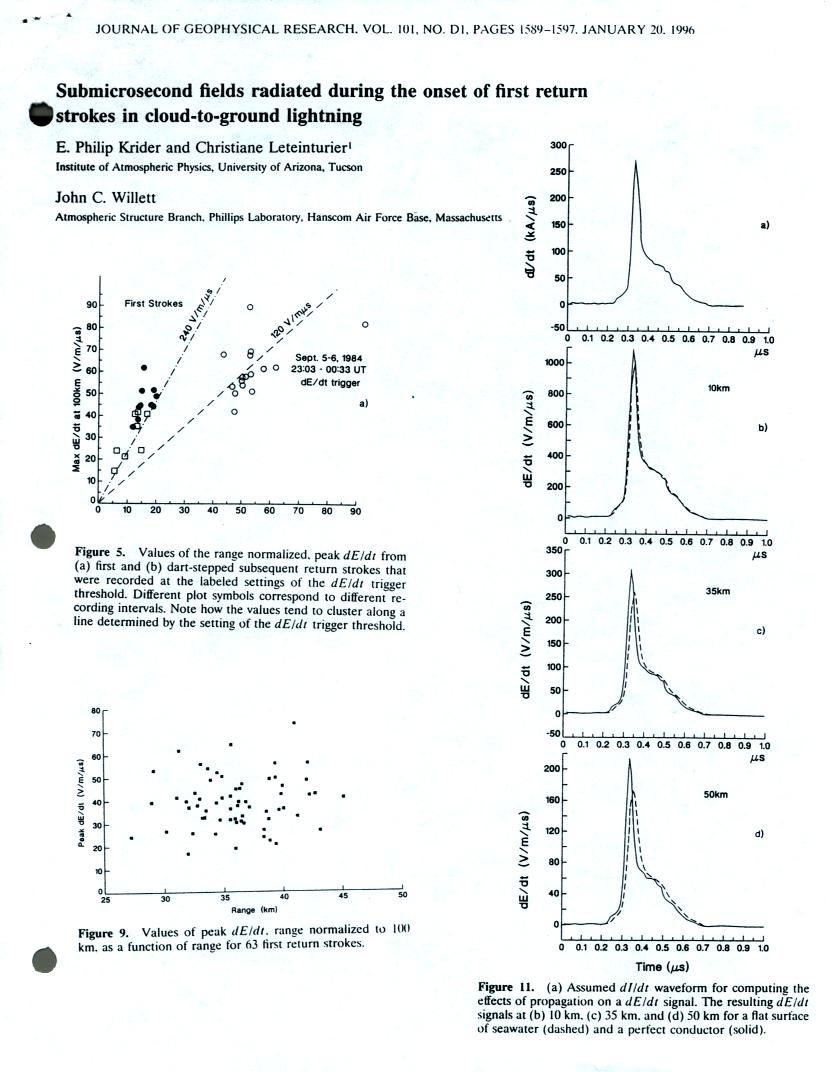
Here is a reference to the paper itself as well as some of the results (this was on a class handout).
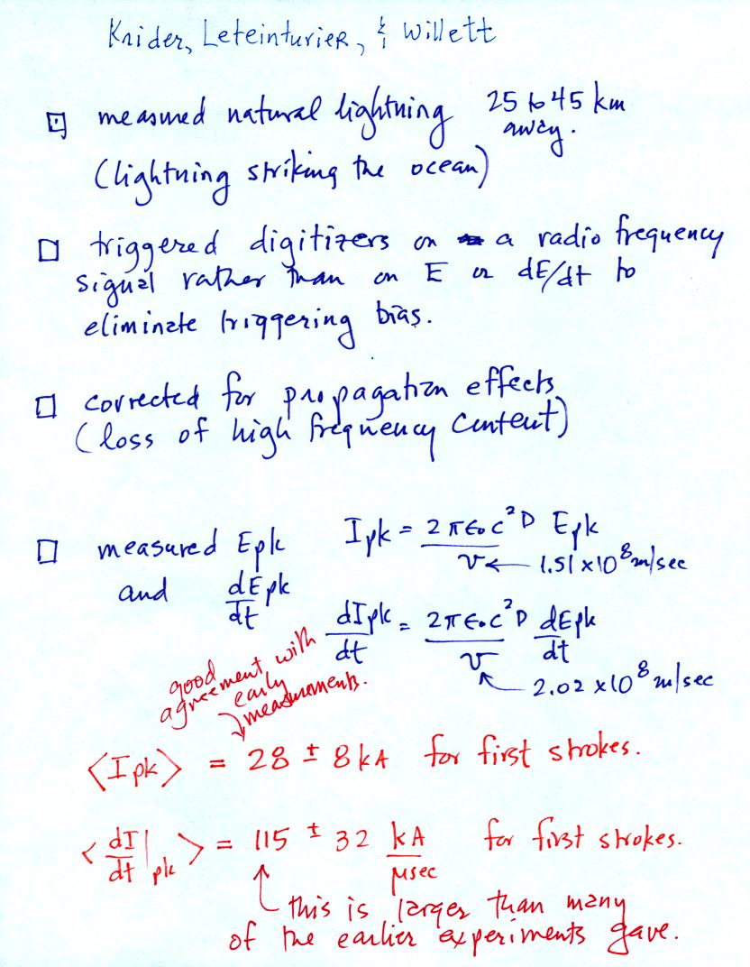
Here are some important points regarding this experiment.
1. Fields from lightning 25 to 45 km away was measured. Propagation between the strike point and the recording station was entirely over salt water so that high frequency signal content was preserved.
2. The recording instumentation was triggered on an RF signal rather than on E or dE/dt to prevent trigger bias.

The plot above shows range normalized dE/dt data versus
range. The dE/dt trigger threshold for a fixed trigger level
setting becomes larger and larger with increasing range. At some
ranges the distribution of measured dE/dt signals will be biased toward
larger signal amplitutdes. At sufficiently large range, it is
possible that none of the dE/dt signals will be large enough to trigger
the recording instrumentation.
3. An atttempt was made to correct for the attentuation of high frequency signal content by propagation over a surface with finite eonductitivty.
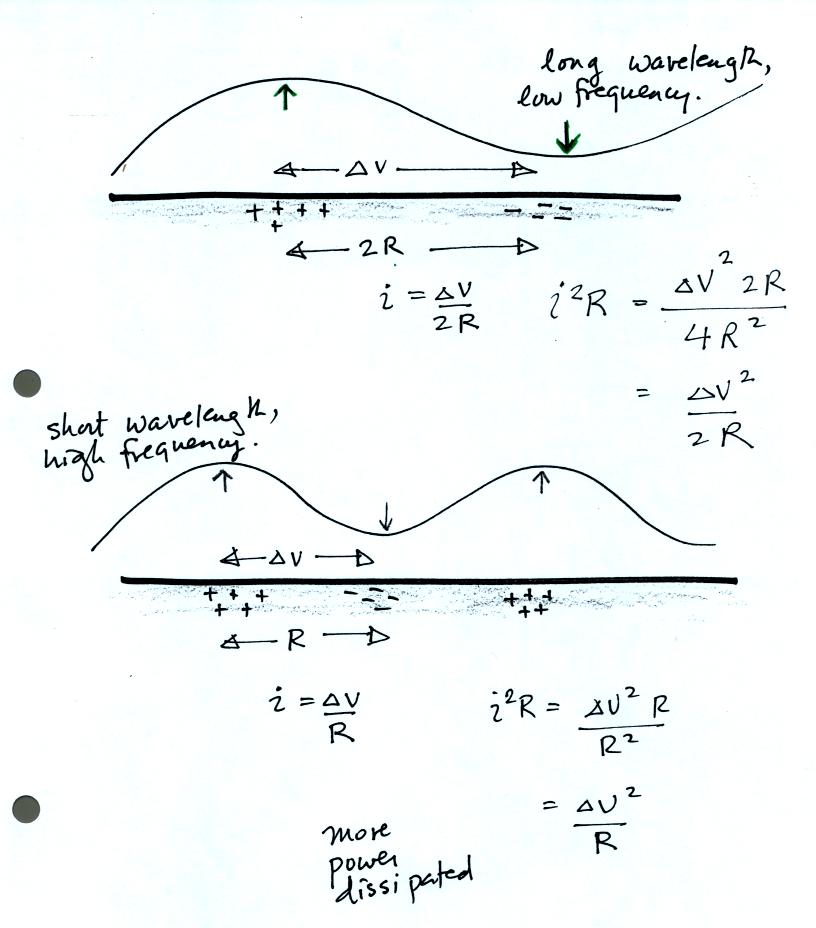
This figure attempts to show why short wavelength, high frequency
radiation undergoes greater attenuation than longer wavelength signals.
Now here's a quick and probably somewhat confusing explanation of how the two wave model can produce a peak and a shoulder in the E field waveform.
We ended the day with a look at some experimental measurements of distant electric radiation fields and estimates of peak I and peak dI/dt values that were derived from them.
Here is a reference to the paper itself as well as some of the results (this was on a class handout).
Here are some important points regarding this experiment.
1. Fields from lightning 25 to 45 km away was measured. Propagation between the strike point and the recording station was entirely over salt water so that high frequency signal content was preserved.
2. The recording instumentation was triggered on an RF signal rather than on E or dE/dt to prevent trigger bias.
3. An atttempt was made to correct for the attentuation of high frequency signal content by propagation over a surface with finite eonductitivty.