A handout
was distributed in class showing how the electric field in the vicinity
of a conducting sphere could be determined by solving Laplace's
equation.
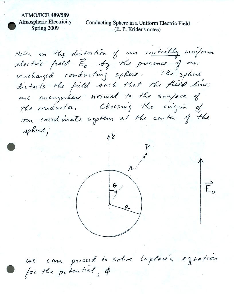
This first page shows the
geometry. Spherical polar coordinates
are used, there is azimuthal symmetry, so the potential and the
electric field will depend on r and theta only.
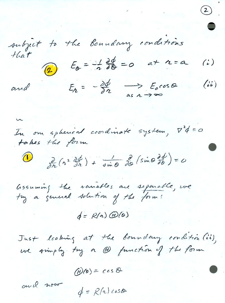
The notes
below add a few details and show how the equation at Point 1 above was
obtained.
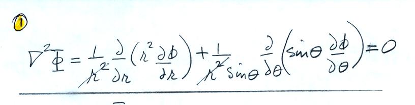
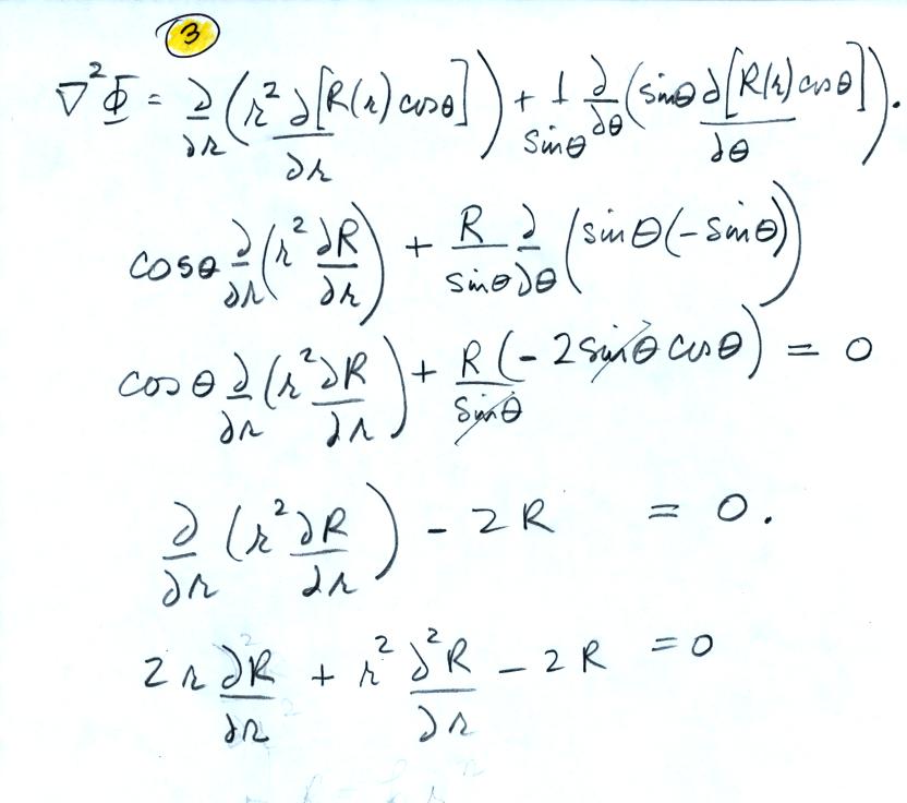
You substitute into the equation
for the Laplacian
in spherical polar coordinates (on a handout distributed in class last
Tuesday). The 1/r2 term cancels.
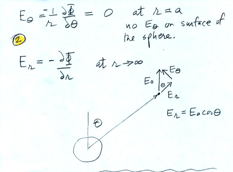
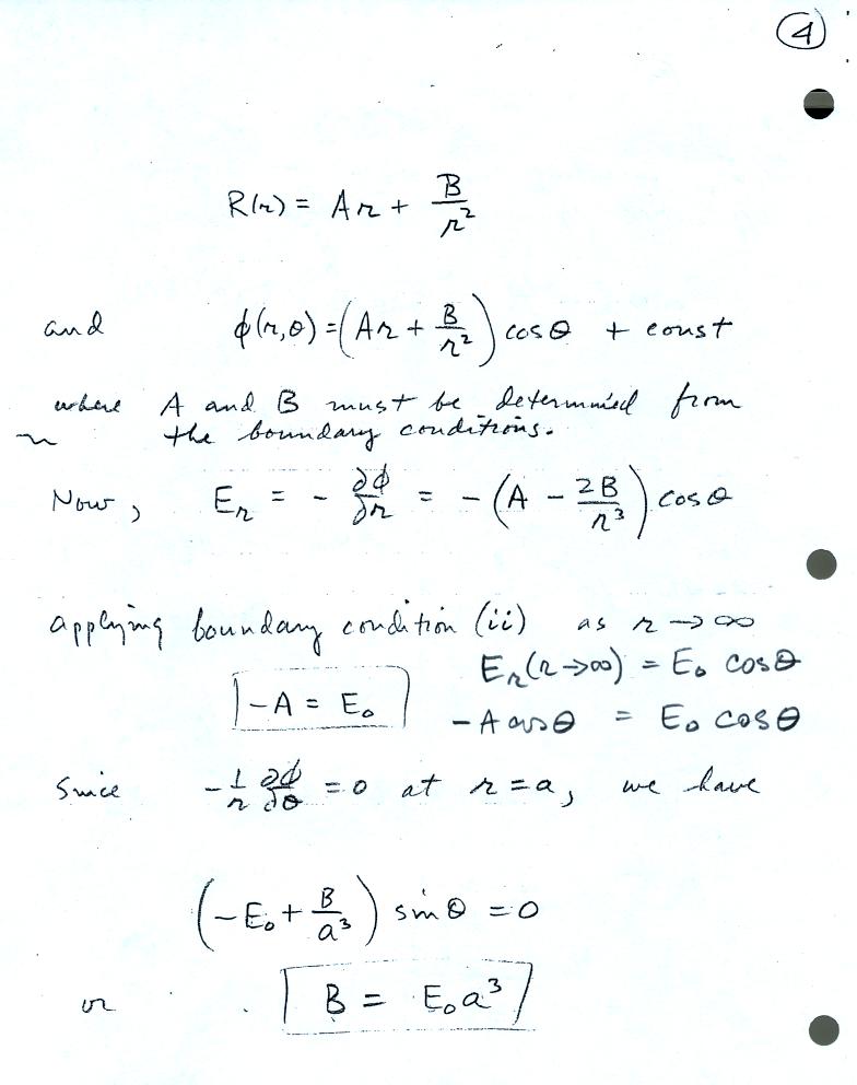
Here is
some additional explanation of the two boundary conditions at Point 2
above.
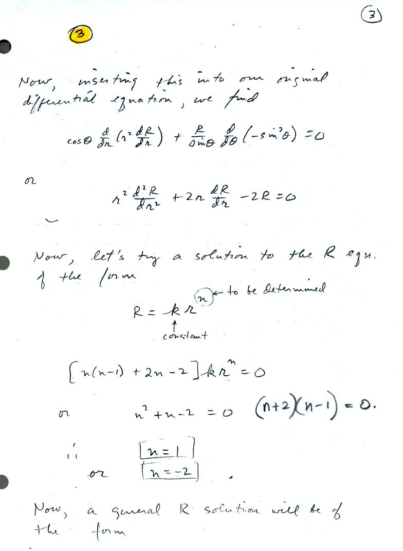
The
following notes fill in some of the missing details in Point 3 above.
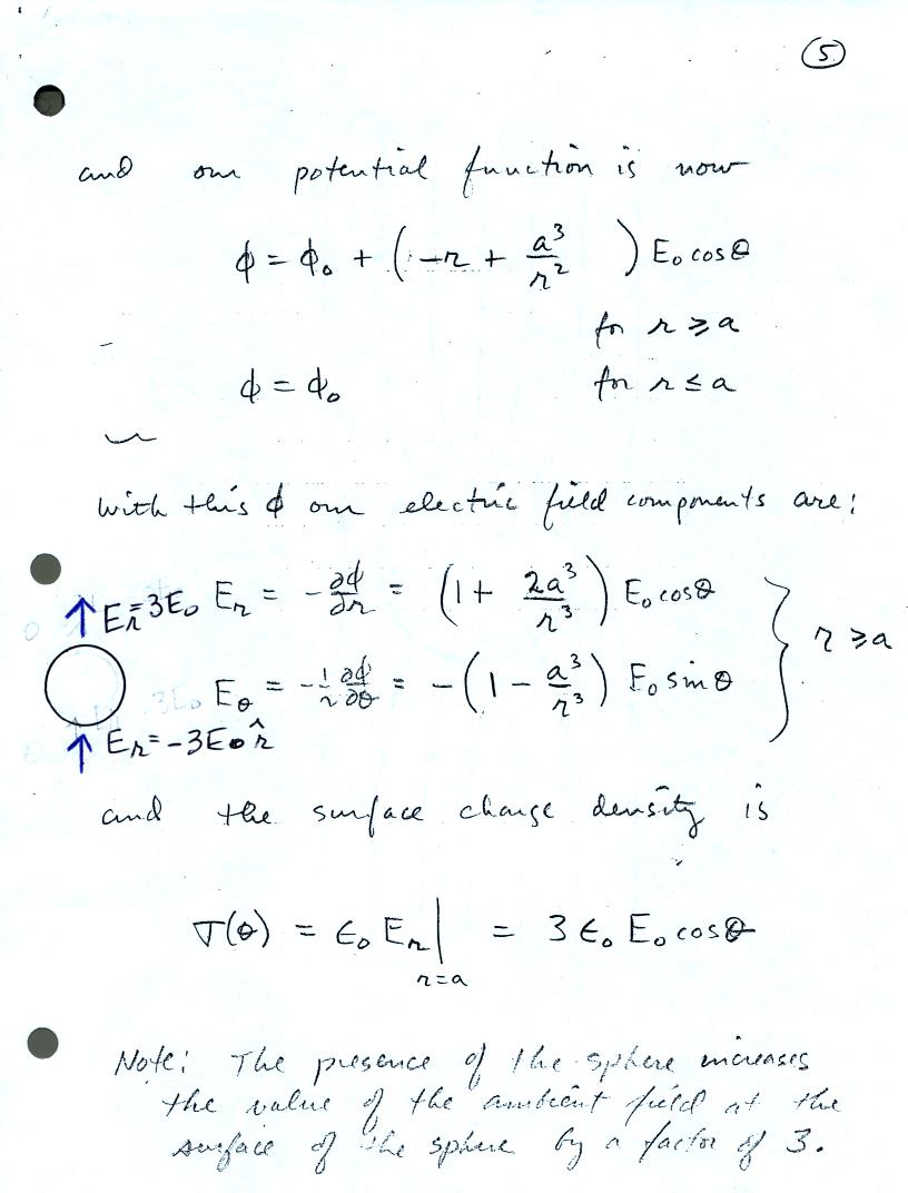
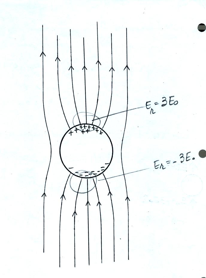
This figure gives you a rough idea
of how the field is changed in the vicinity of the sphere. E
field lines must intersect the sphere perpendicularly. The field is
enhanced (amplified) by a factor of three at the top and bottom of the
sphere.
Enhancement
of
fields by conducting objects is an important concern. In some
cases (we'll look at an example or two later) the enhanced field is
strong enough to initiate or trigger a lightning discharge.
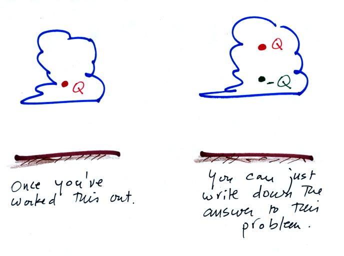
The following handout gives a rough, back-of-the-envelope kind of
estimate of the factor of enhancement.
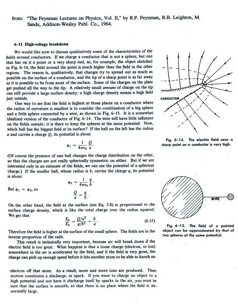
This might require a little
explanation.
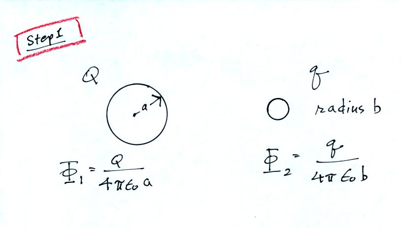
First you write down the potential
at the surface of two conducting spheres of radius a and b, carrying
charges Q and
q.
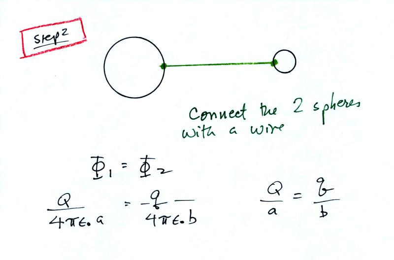
Then you connect the two spheres
with a wire and force the two
potentials to be equal (of course this would cause the charge to
rearrange itself, but we will ignore that).
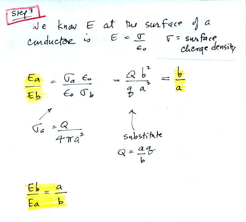
Finally we write down expressions
for the relative strengths of the
electric fields at the surfaces of the two spheres. We see that
the field at the surface of the smaller sphere is a/b times larger than
the field at the surface of the bigger sphere.
Here is a
real example of field enhancement that lead to triggering of a
lightning strike and subsequent loss of a launch vehicle (you'll find
the entire article here)

In this case the rocket body together with the exhaust plume created a
long pointed conducting object. Enhanced fields at the top and
bottom triggered lightning.
Lighning is sometimes triggered at the tops of tall mountains
Note the direction of the branching. This indicates that
this discharge began with a leader process that traveled upward from
the mountain. Most cloud to ground lightning discharges begin
with a leader that propagates from the cloud downward toward the
ground. We will of course look at the events that occur during
lightning discharges in a lot more detail later in the
semester.
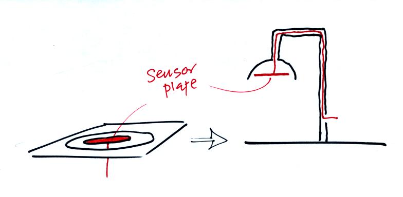
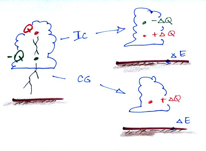
Here's an example of a very
cleverly designed instrument that could be used to measure electric
fields above the ground and inside thunderstorms. Two metal
spheres are attached to a horizontal insulating tube.
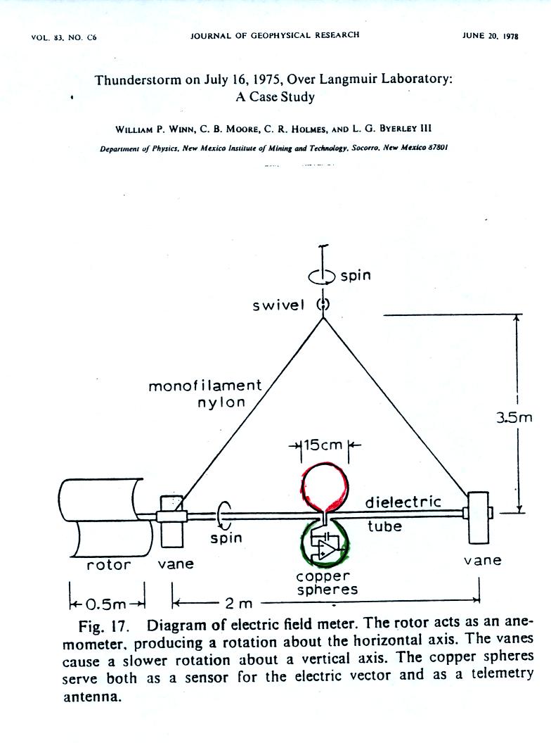
A rotor causes the two spheres
(colored red and
green to distinquish between them) to spin as the balloon moves upward.
As the spheres spin, a current will move back and forth between
them. The amplitude of the current will depend on the charge
induced on the spheres by the electric field.
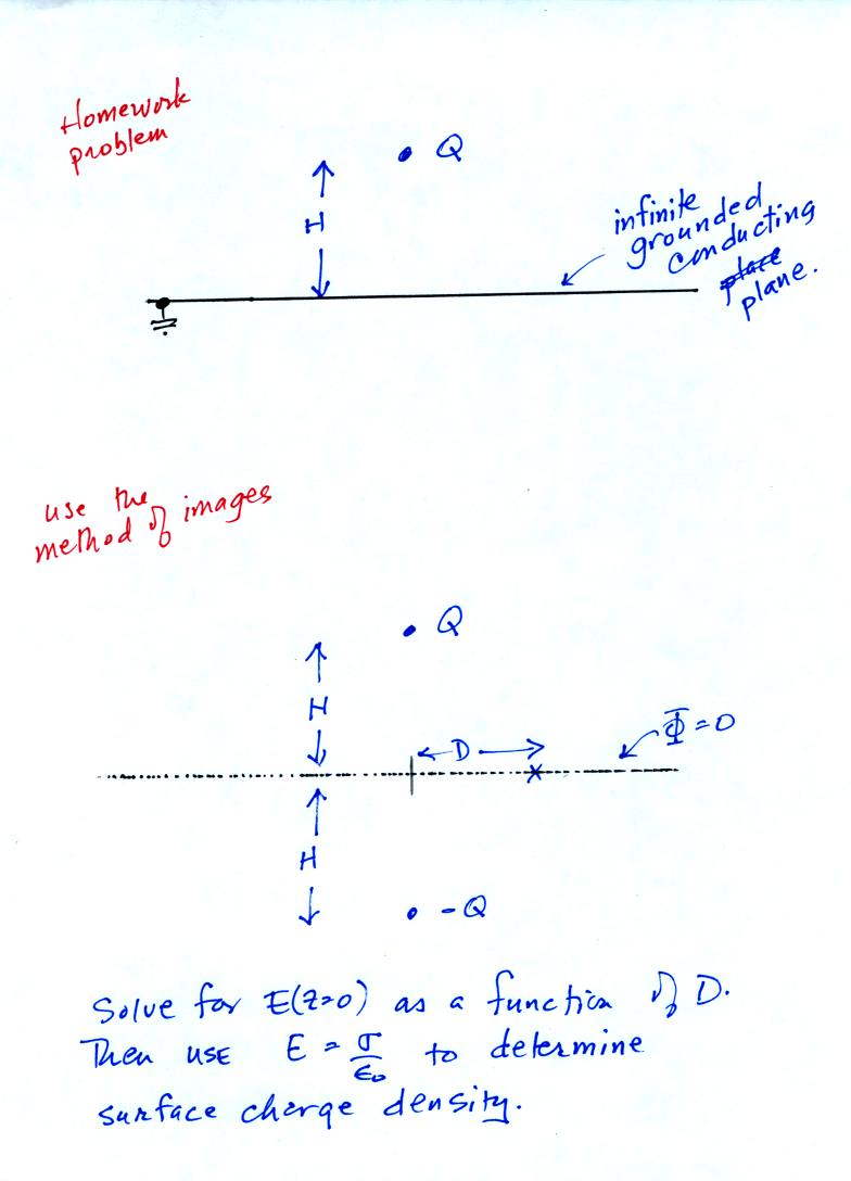
We didn't have time to carefully discuss what follows. We'll come
back to it briefly next Tuesday. I include it here because you do
an essentially identical calculation in Problem #1 on your homework
assignment.
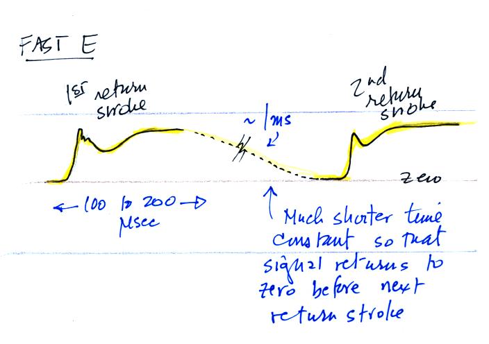
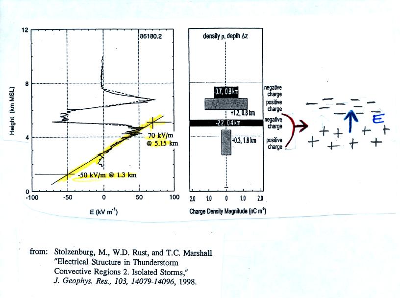
The next figure shows an example of data obtained with an instrument
like this (it is from a different paper). This was on a handout
distributed in class.
The vertical field swings between large negative and positive
values (tens of kilovolts/meter) as the field mill passes through
layers of positive and negative charge in a thunderstorm cloud.
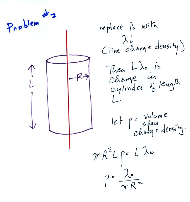
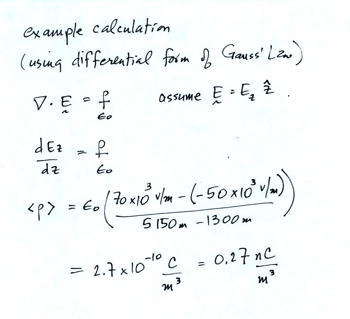
We use the E field data
between 1.3 and 5.15 km altitude below to derive an estimate of the
average volume space charge density in the bottom layer of positive
charge.
The value we obtain (0.27 nC/m3) is in good agreement with the value
given in the paper.