The
list below gives you an idea of the electrical parameters that
were measured and the various types of sensors that were used.

Measurements
of
conductivity versus altitude made on two different days are
shown in two graphs below.
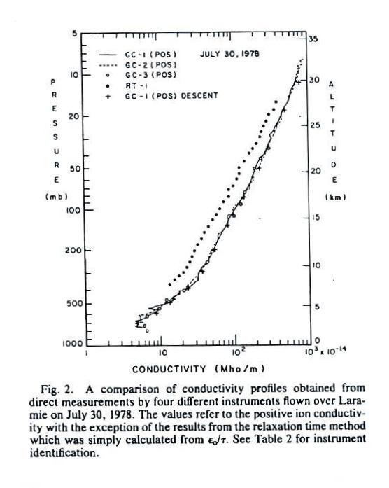
Conductivity values range from about 5 x 10-14
mhos/m at 2 km or so above the ground to about 1000 times
higher than that near 30 km. Note that conductivity is
plotted on the x-axis on a logarithmic scale. The 10 -
30 km portion of the graph appears pretty linear implying
conductivity is increasing exponentially with altitude.
The conductivity values are from just the positively charged
small ions. The notation "GC" in the figure refers to "Gerdien Condenser." The
cylindrical capacitor discussed in the last lecture would be
an example of a Gerdien condenser
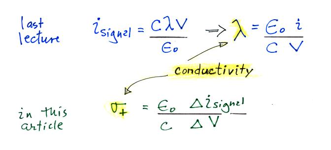
type instrument. Conductivity was estimated using the Isignal/V slope method described in
our last lecture (σ is used in the article instead of λ).
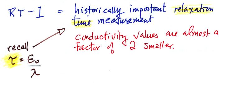
All of the measurements are in good agreement with the exception of the relaxation time
method. This is just the decay time constant we derived
in a previous lecture.
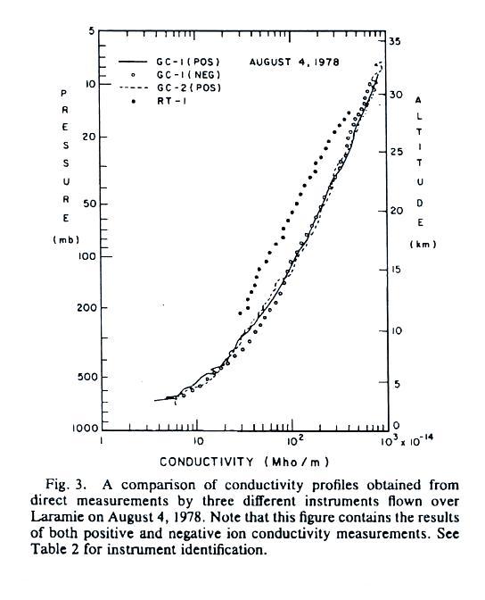
A
second set of conductivity measurements. These include
both positive and negative small ions.
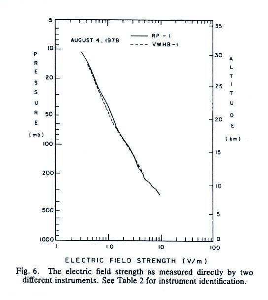
The
next
two plots show measurements of electric field versus altitude
(the same two plots were on the 2nd homework assignment).
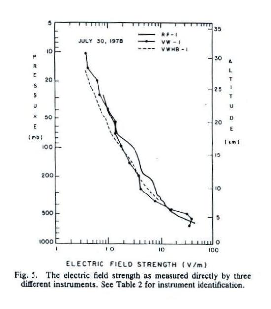
E field values decrease from a few 10s of volts/meter 2 or 3
km above the ground to less than 1 V/m near 30 km (note:
the x-axis values are, from left to right, 0.1, 1.0, 10 and
100 V/m).
The
next plot shows the vertical profile of current density, Jz. Measurements from two
different days are plotted together.
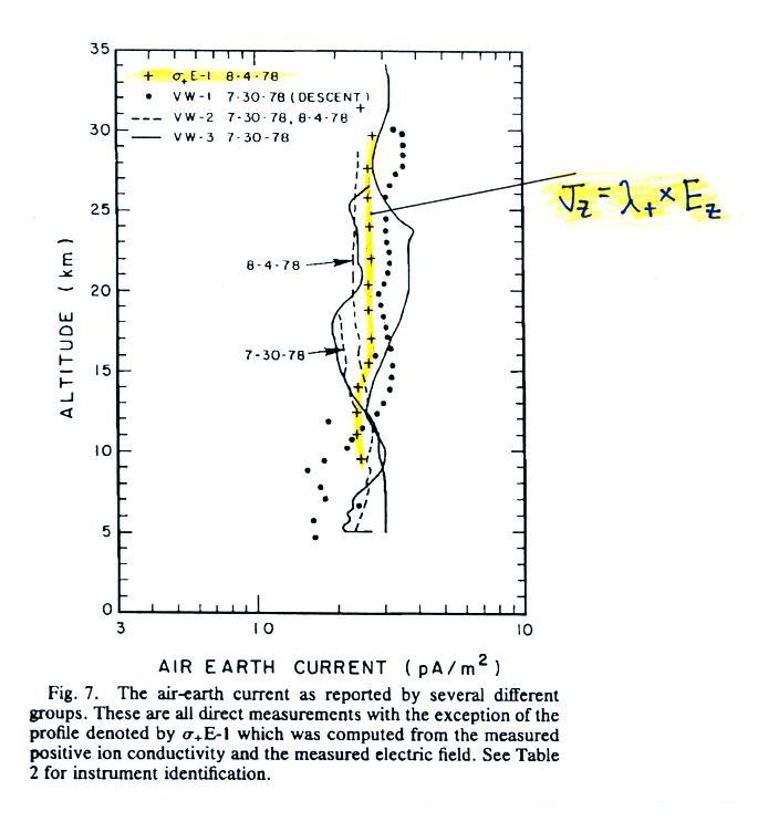
Note first of all that current density does stays fairly
constant with altitude something we expect under steady state
conditions (the x-axis labels, from left to right, are 0.1,
1.0 and 10 pA/m2).
The
yellow curve is the product of electric field and positive
small ion conductivity, all the others are measurements of Jz. You would
expect the measured Jz
(which includes both positive and negative charge
carriers) to to be roughly twice
the positive conductivity times electric field, but it
isn't.
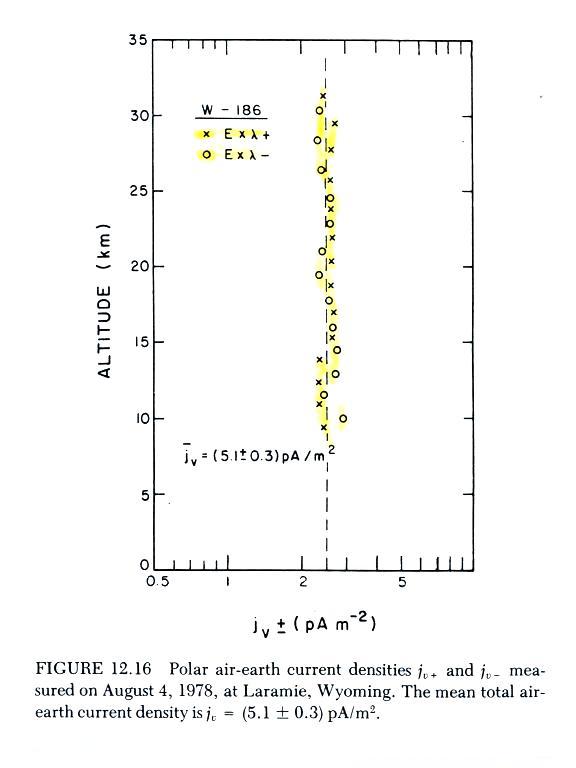
The problem appears to have been corrected in the plot below
which is a reanalysis of the Wyoming data. The plotted
points are conductivity (positive and negative polarity) times
measured electric field. The plotted values cluster
around a value of about 2.5 pA/m2
(note again how uniform Jz
is with altitude). Measured Jz
was about twice this, about 5.1 pA/m2.
The next graph summarizes measurements from a different field
experiment conducted in the North Atlantic ocean.
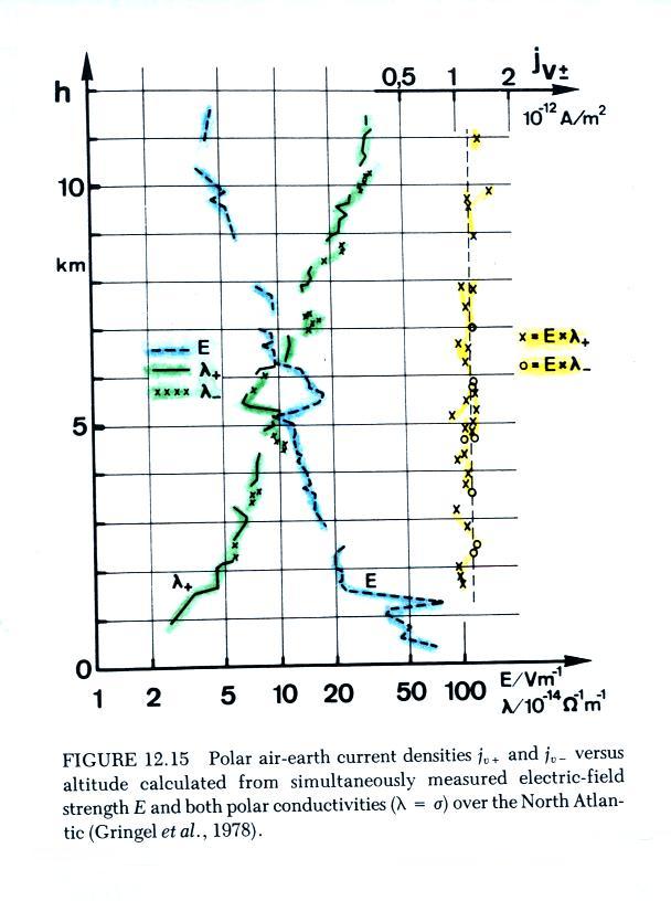
The
plot
shows vertical profiles of E field (highlighted in blue),
measured positive and negative conductivities (green), and the
calculated current density (in yellow, the product of positive
and negative conductivity and measured electric field).
The calculated current density values are clustered around
1.25 pA/m2, the
measured total current density was about twice that, 2.35 pA/m2.
The last two figures above from W. Gringel,
J.M. Rosen, ande D.J. Hofmann,
"Electrical Structure from 0 to 30 km Kilometers," Ch. 12 in The
Earth's Electrical Environment, National Academy Press,
1986. (available online at www.nap.edu/books/0309036801/html/)