Thursday, April 13, 2017

A special guest lecture today from Dr. Donald Huffman (Regents' Professor from the UA Physics department) this morning that covered spectroscopy and ball lightning.  I will attempt to blend together images from his PowerPoint slides and my own notes on lightning spectroscopy.


Class began with a series of demonstrations:  Looking at a tungsten bulb (with a long vertical filament) through a diffraction grating produces a continuum spectrum (all the colors of visible light spread out horizontally).  The spectrum produced by a helium-filled gas discharge tube (a hydrogen source wasn't available) consists of a series of distinct lines, unique to helium.  Without a slit, the spectrum of an extended source, a CFL bulb, produces a series of overlapping images of the bulb.  When a narrow slit is placed in front of the same bulb, distinct lines could be seen in the spectrum.  At some point I will try to duplicate and include photographs of the demonstrations but I'll need to first try to repair my camera.

Slitless and time resolved lightning spectroscopy
A conventional spectrometer is shown in the figure below (viewed from above)


Light from an extended source (a source with large horizontal extent) enters the spectrometer through a narrow vertical slit which is positioned at the focal point of a collimating lens (a diffraction grating could also be used in place of the prism).  The parallel rays of light then passes through the prism and are refracted and dispersed.  These rays are focused onto a detector with a second lens.  The spectrum that is obtained is a multitude of images of the entrance slit, each at a different wavelength, spread out across the detector.  Making the slit narrower makes the spectral features sharper but also cuts down on the brightness of the spectrum.


A schematic diagram of a somewhat simpler "slitless" spectrometer design is shown below (the lenses have been left out of the figure).


Light from a lightning channel passes through both a prism and a diffraction grating and is imaged on film (or a detector of some kind).  An entrance slit is not needed because the lightning channel is essentially already a line source.  The spectrum that you would obtain in this case would be a series of images of the narrow channel at each of the wavelengths emitted by the discharge.  The spectrograph above is different in another respect because it combines both a prism and a diffraction grating.  In a 1961 article in Science, Leon Salanave explains that both a prism and a diffraction grating were used and arranged "so that their respective deviations counterbalance, to make a more 'straight-through' optical system."  The combination of a prism and a diffraction grating is sometimes referred to as a "grism."  Dr. Salanave directed much of the lightning spectroscopic research work done at the University of Arizona for several years.  He is also the author of "Lightning and Its Spectrum " published by the University of Arizona Press in 1980.


Stars are point sources of light so a slitless spectrograph can be used here also.  Spectra of stars in two constellations are shown below:


Slitless spectra of the stars in the Pleiades and Hyades from the textbook shown at right.

Small particles illuminated with a bright light source also act as point sources of slight (the figure below is from Huffman et al., 2016; a full citation and a link to the article are at the end of today's notes)


In the center picture particles on a substrate can be illuminated with either a tungsten source (white light) or a laser or LED source.  The spectrum of the white light reflected (scattered) by the particle could provide information about its composition.  Illumination with ultraviolet (UV light emitted by a laser or LED source) could cause the particle to fluoresce which would provide additional information about the particle.  Again because the particles are small, they act as point sources and a slit in the spectroscope isn't needed.


The photograph at upper left shows the particles.  Panel (b) shows particles illuminated with white light, plus lasers at 650 nm, and 405 nm.  The laser points serve to calibrate the wavelength scale.  Panel (c) shows the scattering spectra of each particle under white light, and panel (d) shows fluorescence spectra excited by 405 nm light.


Lightning spectroscopy
We'll take a quick look at f
ast time resolved lightning spectroscopy.  Spectroscopic measurements have been used to determine some interesting and fundamental properties of the lightning channel such as temperature and pressure.  Also we need to take note of some of the bright spectral features that could be used to detect and locate lightning from a satellite.


(Image credit: Denis Joye from http://spaceplasma.tumblr.com/post/61751774825/lightning-spectra-in-his-celebrated-1704-book)

The image above was most likely captured by placing a diffraction grating in front of the camera lens (look at the lower portion of the spectrum and you will see spectra to the left and right of the channel, a prism would only produce a spectrum on one side of the lightning channel and also I think the order of the colors would be reversed).  Concentrate on the nearly vertical portion of the lightning channel near the center of the picture.  An enlargement of the spectrum to the right of the channel is shown below and some of the emission lines have been identified.


NII refers to singly-ionized atomic nitrogen, NI is an emission from an excited by an unionized nitrogen atom.  H-alpha and H-beta refers to emission lines in the Balmer series of hydrogen atoms (energy level 3 to level 2 and energy level 4 to level 2 respectively).    The hydrogen likely comes mostly from the dissociation of water vapor (H2O) by the lightning discharge.

Here's another implementation of the principle


These images are from an online PowerPoint presentation "Lightning Spectroscopy" by T. Walker, H. Christian, and D. Sentman.  The video camera is a Phantom v710 with a CMOS 1280x800 array with 12 bit dynamic range (in a separate conference publication the resolution was reduced to 1040 x 8 pixels so that 673 k images could be acquired per second).

An example spectrum obtained with the system above from a triggered lightning discharge is shown below.


This image is from the Power Point presentation mentioned earlier.  There is no caption or written description but I believe we are seeing emissions produced during the initial continuous current portion of a triggered lightning discharge.  The vertical trace at left shows the channel current recording at the base of the discharge.  The spectral emissions are probably coming from a short vertical segment of the channel located above the ground but below the top of the wire.
  I believe time is being shown on the vertical axis (in milliseconds?).  Thus we are seeing the time evolution of emissions produced during vaporization of the triggering wire.  The negative numbers might indicate times that occurred before some event later in the discharge such as the initial subsequent return stroke.  The bright green features in the spectra come from vaporization of the copper wire used to trigger the lightning.

High speed video cameras are a fairly recent invention.  Before that time resolved spectra were obtained by isolating a vertical segment of the lightning channel and recording the spectrum on moving film.


The film is shown moving downward in this picture (and sorry that the perspective isn't quite right).  Spectra from two separate return strokes 10s of milliseconds apart, perhaps, have been recorded on the film.  This is essentially what was being done on the newer digital system above except that the spectrum was recorded on successive video frames rather than being smeared out on film.

Here are actual implementations that provide moderate and very fast time resolution (see Krider (1973)).


The rotating drum in the lower figure provides the fastest time resolution (microsecond resolution).  Rapidly rotating drums in streaking cameras are also used in photographic measurements of return stroke velocity.


The next figure shows an actual example of a very fast time resolved spectrum from a return stroke.


Several emission features are identified on this spectrum early in the return stroke discharge (NII denotes a singly ionized nitrogen atom).  You'll find a better quality image in the Krider (1973) paper.  Now what is usually done next is to scan across the film image using a densitometer at say perhaps the level of the green line (i.e. at a time about 10 microseconds after the beginning of the return stroke). 


Here is an example of a "digitized" spectrum.  Film's response to light is nonlinear, so the film must be carefully calibrated.  Film also reacts differently to short bright impulses of light than it does to longer duration low amplitude light signals.  So that effect must also be considered.

Six emission lines in the NII(5) multiplet spectrum above have been identified.  I am not familiar enough with spectroscopy and quantum mechanics to be able to say for sure what precise states and transitions cause these features

but I'm guessing it looks something like shown here.  Transitions from 2 slightly different energy levels in an excited state to 1 of 3 levels at a lower energy state could produce emissions of 6 slightly different wavelengths.

In any event it is the relative amplitudes of lines in a multiplet group that can be used to estimate lightning channel temperature.  The procedure is described below.  Our goal is not to try to understand all the steps but rather to get a flavor for the procedure or method.

The first assumption made is that the number of atoms in a particular energy level can be described using a Maxwell-Boltzmann distribution This is where temperature plays a role.


Nn is the number of atoms in energy level n, N is the total number of atoms.


The intensity of the emission produced by transitions from energy level n to r is shown above. 

Now we will look at the ratio of measured intensities from two different transitions: n to r and m to p

It is these transition intensities that can be measured on the fast time resolved lightning spectra.  Note that many of the parameters cancel.  This is fortunate because some of them (such as the geometric factor) might be difficult to determine.  Solving for temperature yields

Often what is done is that several determinations of temperature are made using different combinations of lines in the multiplet group and an average is computed.  In the case of the NII(5) multiplet 5 ratios could be computed: 4630/4601, 4630/4607, 4630/4613, 4630/4621, and 4630/4643.

 
Lightning channel thermodynamic properties derived from spectroscopic measurements
The next several figures shown some of the results of these spectroscopic measurements and analyses.


Concentrations of NIII (doubly ionized atomic nitrogen), NII (singly ionized atomic nitrogen), and NI (neutral atomic nitrogen) early in a return stroke discharge.  NII is initially the most abundant species and is used in spectroscopic determinations of peak temperature in the return stroke channel.


Estimate of peak return stroke channel temperature.  The value approaches 30,000 K which is approximately 5 times hotter than the surface of the sun (6000 K).

Here are estimates of channel pressure.  This requires a measurement of temperature and probably density (including electron density from the ionized air molecules).  The high pressures in the lightning channel cause the air to explode outward (a shock wave decays quickly to a sound wave).   It is the sound of that explosion that we ultimately hear as thunder.


Properties and characteristics of "ball lightning"
Next we'll consider the topic of ball lightning
spectroscopy which will play an important part in this discussion also.  And we should note that "ball lightning" is not really lightning, rather a phenomenon produced by lightning.


Some ball lightning references mentioned in class and relevant to the discussion that follows are listed below.  Links to all of these articles are included at the end of today's notes.


Pay particular attention to the chronology.  We'll look first at a theory that might explain the phenomenon of ball lightning (the Abrahamson and Dinniss (2000) paper).  This was followed by a laboratory experiment that seemed to produce ball lightning like luminous spheres (Paiva et al., (2007).  Finally we'll look at a recent recording of a spectrum attributed to ball lightning (Cen et al., (2014)) that contains some of the features predicted in the earlier theoretical work. 

This is the also the way one likes to see research proceed - a theory that is later supported by experiment rather than development of a theory seeks to explain new experimental results.


A proposed mechanism for the formation of ball lightning.
Here is the mechanism suggested by Abrahamson and Dinniss for the formation of ball lightning: "When normal lightning strikes soil, chemical energy is stored in nanoparticles of Si, SiO or SiC, which are ejected into the air as a filamentary network.  As the particles are slowly oxidized in air, the stored energy is released as heat and light."


Proposed formation of "Ball Lightning" after Abrahamson and Dinniss (2000)
Electron microscope photograph of nanoparticle chains from the Abrahamson and Dinniss (2000) article.  The particles were produced by a 14.9 kV discharge to silt loam soil containing carbon.

Abrahamson and Dinniss were not able to produce any luminous balls, "... the soil sample was always completely blown away in the radial direction."  The cylindrical fulgurites produced by lightning are often hollow and might confine the nanoparticles produced by the discharge.


Photograph of a hollow fulgurite (and its reflection)
Details of proposed "Ball Lightning" production

In the fulgurite cavity, silicon dioxide SiO reacts with carbon to form ionized silicon and carbon monoxide.  The silicon ions quickly form chains that then get tangled together to form a larger "ball."  
               
SiO2 + 2C ---> Si+ + 2CO

The ions emit light as they oxidize and decay to a lower energy state.


A sketch of the structure of aerogel
A photograph of aerogel

A close but stable analogy is aerogel which is made up of strands of silicon dioxide, SiO2 .

Production of ball-lightning-like luminous balls in a laboratory


Schematic and description of the apparatus used to make ball lightning like spheres in a laboratory (from Paiva et al. (2007)).  The balls were produced by striking a silicon wafer with an electric arc.  Links to several short videos that show the glowing balls produced in these laboratory experiments are listed below (the list is from:
http://ftp.aip.org/epaps/phys_rev_lett/E-PRLTAO-98-047705 )

What may be the first spectrum of ball lightning


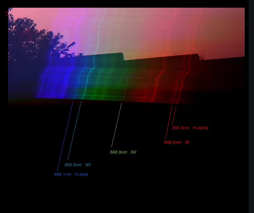
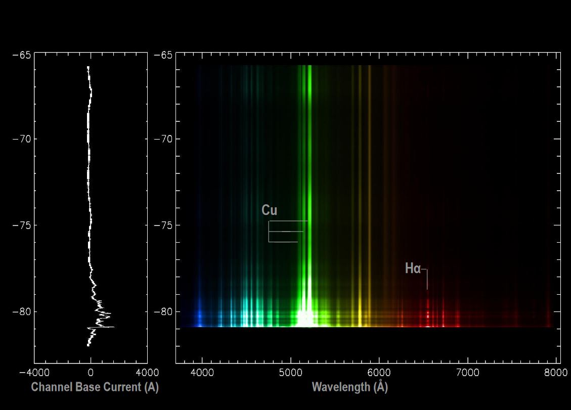
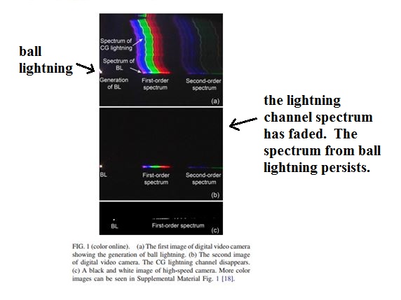
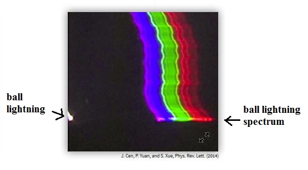
A figure from Cen et al. (2014) with what may be the first spectrum of ball lightning (above left).  The spectrum of the ball lightning (BL) can be seen at the very bottom of the channel.  The spectrum above is from the lightning channel above the ground.  Note that light from the "ball lightning" persists well after the spectrum from the channel above has faded.  The discharge was 0.9 km away and the ball lightning emissions persisted 
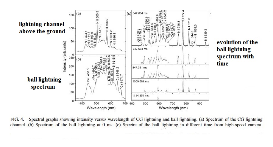
for 1.64 seconds.  A somewhat larger view of the bottom of the lightning channel and the ball lightning spectrum (from Ball (2014))


The two graphs on the left side of the figure above (adapted from Cen et al. (2014)) show spectra from the natural lightning channel (upper portion) and from the ball lightning at the bottom of the channel.  The two spectra are very different.  We see only NII (singly ionized nitrogen) emission features coming from the lightning channel.  The ball lightning spectrum contains emissions from iron (Fe), silicon (Si), and calcium (Ca).  Note the ionized silicon line (Si II) at 505.5 nm.

So What's in the future?
Dr. Huffman concluded his lecture with a short video segment showing the apparatus (see photograph below) that he has been using for many years (decades) to produce carbon smoke.  It was from this carbon smoke that he was able to separate and thereby first find a means of producing C60
.  The same apparatus could also be used to carefully investigate silicon's proposed role in the formation of ball lightning.


References:

Background information on Dr. Huffman and the discovery of C60
Donald R. Huffman, "Solid C60", Physics Today, 44, 22-29, 1991.
BBC program Horizon 1996 "Molecules with Sunglasses"


Topics covered in today's class
L.E. Salanave, "The Optical Spectrum of Lightning," Science, 134, 1395-1399, 1961.

T.D. Walker and H.J. Christian, "Novel Observations in Lightning Spectroscopy," XV International Conference on Atmospheric Electricity, Norman OK, 2014.

D.R. Huffman, B.E. Swanson, and J.A. Huffman, "A wavelength-dispersive instrument for characterizing fluorescence and scattering spectra of individual aerosol particles on a substrate," Atmos. Meas. Tech., 9, 3987-3998, 2016.

E.P. Krider, "Lightning Spectroscopy," Nuclear Instruments and Methods, 110, 411-419, 1973.

W. Cawood and H.S. Patterson, "A Curious Phenomenon shown by Highly Charged Aerosols," Nature, 128, 150, 1931.

J. Abrahamson and J. Dinniss, "Ball lightning caused by oxidation of nanoparticle networks from normal lightning strikes on soil," Nature, 403, 519-521, 2000.

G.S. Paiva, A.C. Pavao, E.A. de Vasconcelos, O. Mendes, Jr., E.F. da Silva, Jr., "Production of Ball-Lightning-Like Luminous Balls by Electrical Discharges in Silicon," Phys. Rev. Lett., 98, 2007.

J.D. Hill, M.A. Uman, M. Stapleton, D.M. Jordan, A.M. Chebaro, C.J. Biagi, "Attempts to create ball lightning with triggered lightning," J. Atmos and Solar-Terrestrial Physics, 72, 913-925, 2010.

J. Cen, P. Yuan, and S. Xue, "Observations of the Optical and Spectral Characteristics of Ball Lightning," Phys. Rev. Lett., 112, 2014

P. Ball, "First Spectrum of Ball Lightning," Physics, 7, 5, 2014.

B.M. Smirnov, "The properties and the nature of ball lightning," Physics Reports, 152, 177-226, 1987.

The laboratory produced "Ball Lightning" videos can be found at:
http://ftp.aip.org/epaps/phys_rev_lett/E-PRLTAO-98-047705