Tue., Aug. 29, 2006
The Experiment #1 materials were handed out at
the beginning of class today. Start
the experiment at a time when you will be able to check it every few
hours for part of the day (once it is underway it will slow down and
you will not need to monitor it so frequently). Once you have
collected all of your data, return the materials and pick up the
supplementary information sheet. If you weren't able to check out
the materials today, there may be a few extra kits still available on
Thursday.
The first 1S1P Report assignment was made
in class today. You can choose from 4 topics. You can write one
or two reports (or no reports at all, though you won't receive any
credit in that case and your grade might ultimately suffer).
Reports are due at the beginning of class on Monday Sept. 11. Be
sure to review the rules governing
1S1P reports.
I forgot to show the forecast path of Tropical Storm Ernesto issued by
the National Hurricane Center.
Ernesto is now expected to travel northward along a
large portion of the east coast of Florida. Ernesto is predicted
to
pass very close to the Kennedy Space Center and NASA may move the space
shuttle from the launch pad back into the Vehicle Assembly Building for
protection. Meanwhile, in the Pacific, tropical storm John is
forecast to pass close to the southern tip of Baja California where it
could move moisture up into our area and influence our weather by the
end of the week.
Last
week we saw that combustion of fossil fuels and deforestation were
causing the atmospheric concentration of carbon dioxide to
increase. This in turn might be the cause of a 0.7o to
0.8o C
increase in global annual average surface temperature that has observed
over the past 150 years or so.
Today we looked very briefly at some of the natural changes in climate
that have occurred on the earth.
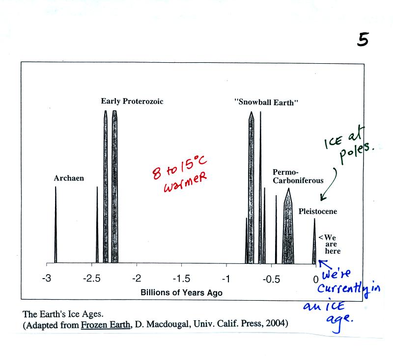
You
might be surprised to learn that the earth is currently in an ice
age, one that began about 2 million years ago. This is one of
several
ice ages thought to have occurred in the past (the figure above is on
p. 5 in the photocopied class notes). Ice is found at the N. and
S. Poles during these ice ages. The poles were ice free during
the long periods in between ice ages. Some scientists believe the
earth's oceans
froze over completely during the coldest ice ages; the name "snowball
earth" is used to describe this occurrence.
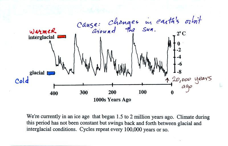
We are
actually living in a relatively warm part of the current ice
age. These warm periods are called interglacial periods. In
between are colder glacial periods. The most recent glacial
period ended about 20,000 years ago. 1 or 2 mile thick ice sheets
covered portions of the norther U.S. during the last glacial
period. An ice
sheet animation shows the
shrinkage of the ice sheets at the end of the last glacial period.
Changes in the shape of the
earth's orbit around the sun and changes in the direction and amount of
tilt of the earth are though to be the cause of the climatic changes
shown in the figure above. Note there is almost a 10o
C
difference in temperature between the warmest and coldest periods.
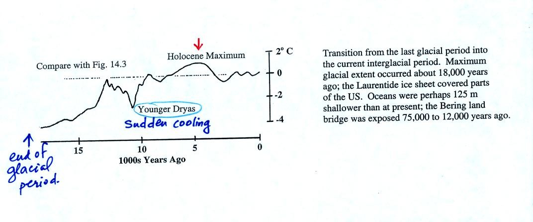
The figure above shows the changes in temperature that occurred as the
earth moved from the most recent glacial period into the current
interglacial period. The Younger Dryas event identified above was
a large and sudden drop in temperatures that interrupted the
warming. Scientists are very interested in abrupt and somewhat
unexpected changes like this. The warm up at the end of the
Younger Dryas period took
only 40 to 50 years, a very sudden change in climate. Note the
Holocene maximum, roughly 5000 years ago, coincides roughly with the
appearance of cities and
the beginning of agriculture.
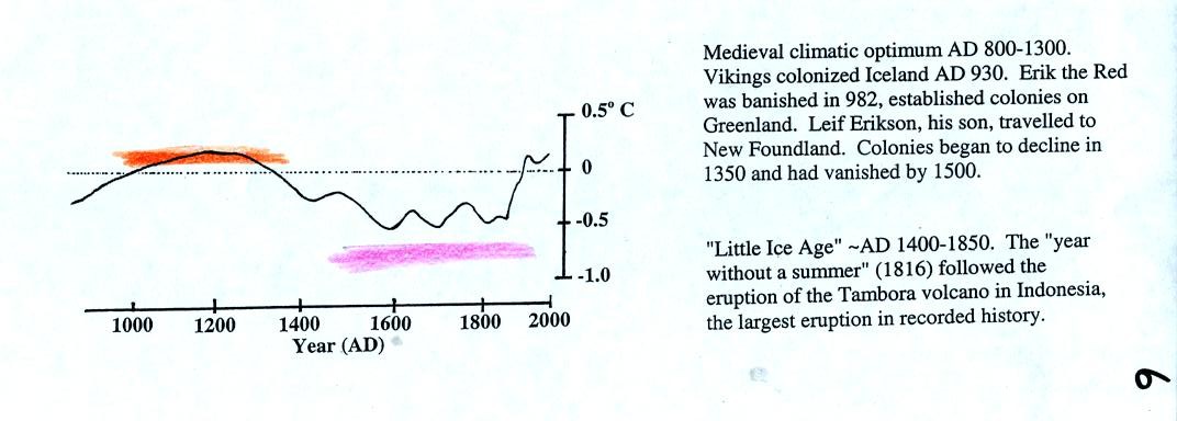
During a
shorter warm period, the medieval climatic optimum, the
Vikings established colonies in New Foundland. These colonies
were abandoned when the climate began to cool and Europe entered a
period known as the Little Ice Age.
Larger volcanic eruptions, like the Tambora volcano mentioned above,
can sometimes cause a short duration change
in climate. These eruptions send small particulates into the
stable stratosphere where they can reflect incoming
sunlight. Probably the best recent example is the Mt. Pinatubo
eruption in June 1991. This caused the global annual average
surface
temperature to cool about 0.5oC. See pps 387 & 389
in
the 4th ed. of the text (p. 385 in the 3rd ed.).
Next we
looked at some predictions for the next 100 years.
Scientists use computer models to predict future climate. They
incorporate mathematical descriptions of the atmosphere and atmospheric
processes into their models. They must also make assumptions
about how human population will grow in the future and how people will
use energy.
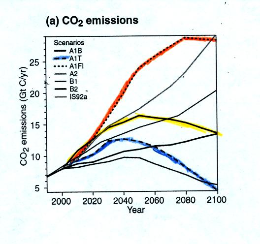
The curves in the next 4 figures assume that there will be rapid
growth of the world economy, that global population will peak in mid
century and
will begin to decline thereafter, and that new and efficient
technologies will be adopted quickly by the world economy.
Three assumptions are made concerning energy sources. The first
(curve A1F1) assumes that fossil fuels will supply most of the energy
needs throughout the period. You can see (orange curve) in the
first figure below that
CO2 emissions are then predicted to grow throughout most of
the next
century. A much better scenario (curve A1T in blue) would be to
assume that a quick
switch to alternative sources of energy is made. In this case CO2
emissions peak fairly early in the next century and then begin to
decrease. The yellow curve lies between these two extremes.
A1F1 - Fossil
fuel intensive (in orange and a "worst case" scenario)
A1B - balance of all energy sources (yellow)
A1T - non fossil fuel energy
sources (in blue and a "best case" situation)
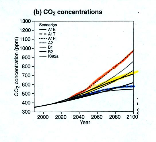
CO2 concentration is
now about 375 ppm. The
figure above
shows CO2 concentrations in 2100 given the three scenarios
above.
In the worst case scenario CO2 concentration would increase
to more
than 900 ppm. In the best case situation CO2
concentration would
increase to about 500 ppm.
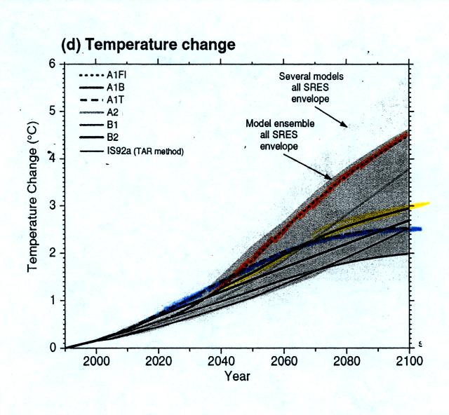
Global average surface
temperatures would increase 2.5o to
about 4.5o C
by 2100 depending on the fuel usage scenario. Some regions would
warm more than this, others less. The figure below shows the 0.3
to 0.5 m expected rise in sea level that would occur as temperatures
began to rise and ice sheets and glaciers began to melt.
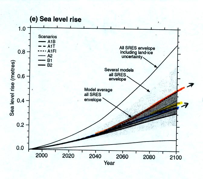
Note that the rising in sea
level is still headed upward at the end of
this period. The melting of the ice starts slowly. Once it
gets started it will then continue for some time even once the warming
stops.
That will end our brief coverage of climate change. We will learn
much more about how the greenhouse effect works when we get to Chapter
2 in the text. Three of the four 1S1P Assignment #1 topics cover
different aspects of climate. You can read more about natural
changes in climate in Topic #2, the causes of natural climatic changes
in Topic #3, and the possible consequences of global warming in Topic
#4.
The four figures above are from "Climate Change 2001: The
Scientific Basis," published by the Intergovernmental Panel on Climate
Change. This and other reports is available online at www.ipcc.ch
At this
point we took a brief detour and had a look at Experiment #1.
With this and the other experiments you will receive most or all of the
materials you need to complete the experiment, a description of what
should go into your report, instructions that tell you how to perform
the experiment, and a data collection sheet.
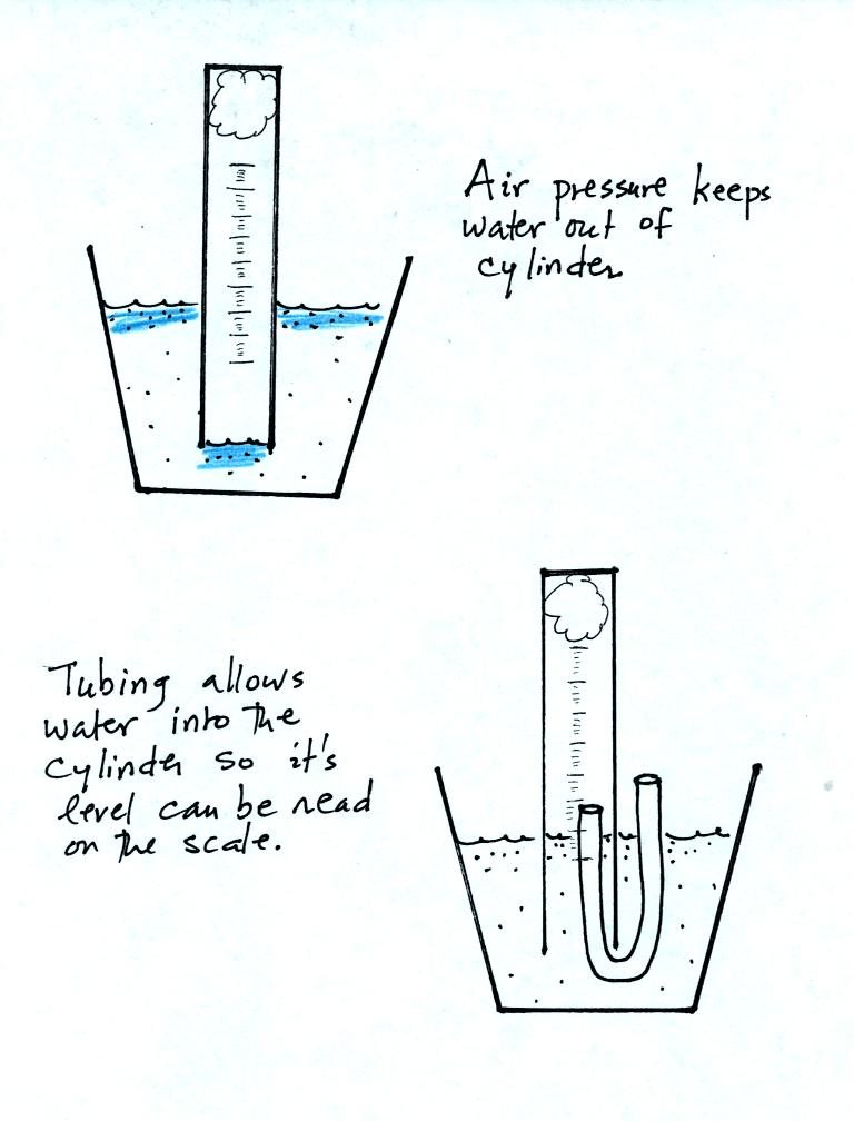
The object of Experiment #1 is to measure the percentage concentration
of the oxygen in air. Basically you moisten a piece of steel
wool, stick the steel wool into a graduated cylinder, and turn the
cylinder upside down and immerse the open end in a cup of water.
As the next figure shows you need to use a small piece of flexible
tubing so that water enters part way into the cylinder so that the
water level can be read on the cylinder scale.
Be sure to remove the tubing once the water level can be
read on the
cylinder scale. The air sample in the cylinder is now sealed off
from the rest of the atmosphere. The oxygen in the air sample
will react with the steel wool to form rust. As oxygen is removed
from the air sample, the air sample volume changes.
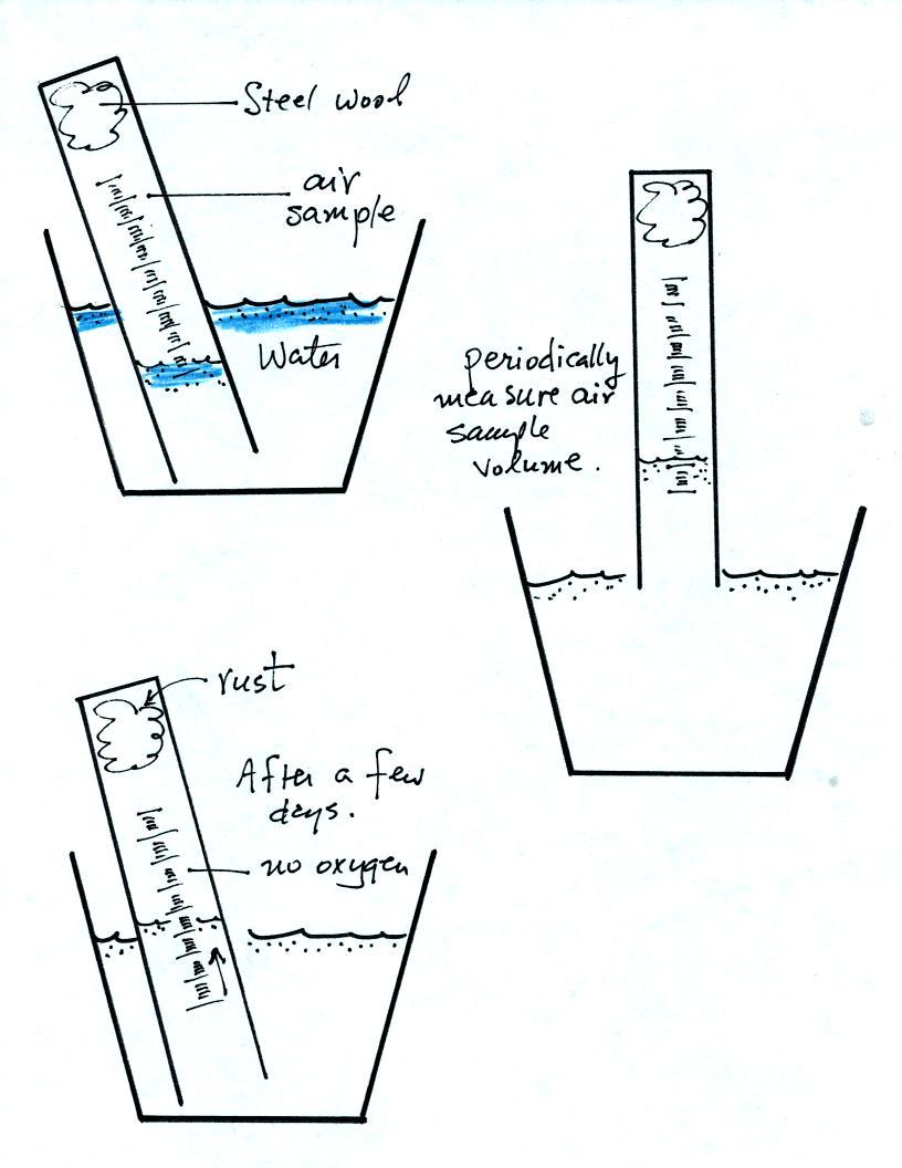
The reaction between the oxygen and the steel wool sometimes
happens in
a day or two. Other times it may take several days. You
will periodically need to record the time and the air sample volume (
you read the water level on the cylinder scale). Be sure you do
not lift the open end of the cylinder out of the water. That
would break the seal and you would need to restart the experiment.
Eventually the air sample volume will stop changing; all of the oxygen
has been removed from the air sample and the experiment is over.
You will receive a supplementary information sheet when you have
returned your materials. You don't have to return the rusty piece
of steel wool - throw it away. Don't worry about trying to clean
the rust stains off the inside of the cylinder.
We next
began our coverage of three of the main air pollutants.
You'll find lots of detailed information about pollutants in Tucson and
Pima County at the Pima County
Department of Environmental Quality webpage. The US Environmental Protection Agency also
has a large amount of information about this topic.
We'll start with sulfur dioxide and finish up with carbon monoxide and
ozone in our next class.
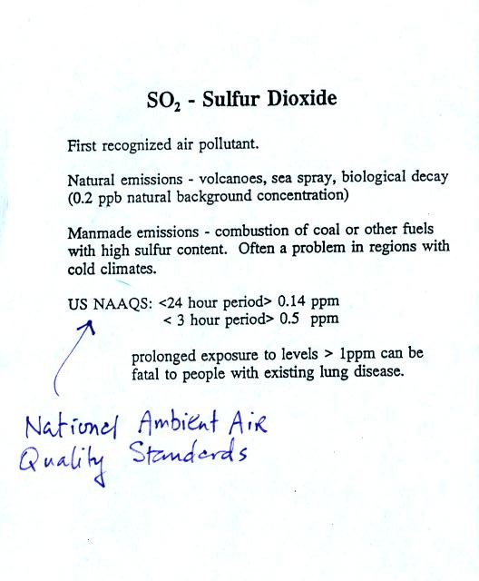
Sulfur dioxide is produced by the combustion of sulfur
containing
fuels such as coal. Combustion of fuel also produces carbon
dioxide and carbon monoxide. People probably first became aware
of sulfur dioxide because it has an unpleasant smell. Carbon
dioxide and carbon monoxide are odorless.
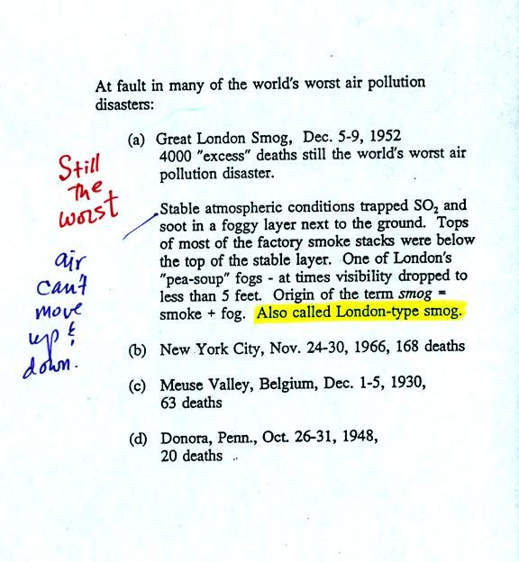
The Great London smog is still the deadliest air pollution event in
history. A stable air layer next to the ground can't mix with
cleaner air above.
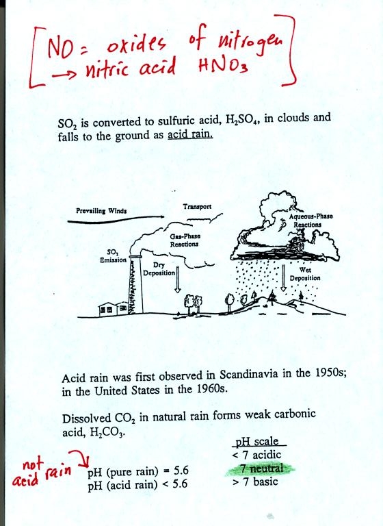
Acid rain often falls hundreds or
thousands of miles away from the
source of the SO2. Coal fired factories and electric
power plants
in the Ohio River Valley could produce acid rain in New England and
Canada. Acid rain in Scandinavia could be the result of SO2
emissions in England and Belgium.
An acid rain demonstration was
performed in the
last 15 minutes of class to give you a general idea of how acid rain is
produced. Carbon dioxide rather than SO2 was bubbled
through
Tucson tap water. The tap water is initially slightly basic (pH
> 7). Dissolved CO2 however turned the tap water
acidic.