Thursday Feb. 7, 2008
Assignment #1 1S1P reports were
collected
at the start of class. You can turn in up to two reports next
Thursday (Feb. 14).
Be sure to return your Experiment #1 materials this week, your report
is due next Tuesday. The first Optional
Assignment is also due next Tuesday.
We'll
finish up learning about how weather data is plotted on surface weather
maps using the station model notation. We didn't have time to
learn about decoding the pressure data.
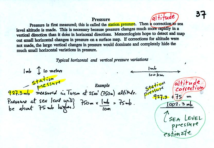
Meteorologists hope to map out small horizontal pressure
changes on
surface weather maps (that produce wind and storms). Pressure
changes much more quickly when
moving in a vertical direction. The pressure measurements are all
corrected to sea level altitude to remove the effects of
altitude. If this were not done large differences in pressure at
different cities at different altitudes would completely hide the
smaller horizontal changes.
In the example above, a station
pressure value of 927.3 mb was measured in Tucson. Since Tucson
is about 750 meters above sea level, a 75 mb correction is added to the
station pressure (1 mb for every 10 meters of altitude). The sea
level pressure estimate for Tucson is 927.3 + 75 = 1002.3 mb.
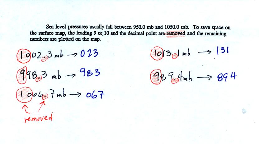
To save room, the leading 9 or 10 on the sea level pressure
value and
the decimal
point are removed before plotting the data on the map. For
example the 10 and the . in 1002.3 mb would be removed; 023
would be plotted on the weather map (to the upper right of the center
circle). Some additional examples are shown above.

When reading pressure values off a map you must remember to
add a 9 or
10 and a decimal point. For example
138 could be either 913.8 or 1013.8 mb. You pick the value that
falls between 950.0 mb and 1050.0 mb (so 1013.8 mb would be the correct
value, 913.8 mb would be too low).
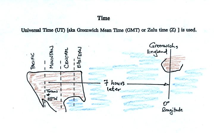
Another
important piece of information that is included on a surface weather
map is the time the observations were collected. Time on a
surface map is converted to a universally agreed upon time zone called
Universal Time (or Greenwich Mean Time, or Zulu time).
That is the time at 0 degrees longitude. There is a 7 hour time
zone difference between Tucson (Mountain
Standard Time year round) and Universal Time. You must add 7
hours to the time in Tucson to obtain Universal Time.
Here are some examples:
8 am MST:
add the 7 hour time zone
correction ---> 8:00 + 7:00 = 15:00 UT (3:00 pm in Greenwich)
2 pm MST:
first convert 2 pm to the 24 hour
clock format 2:00 +12:00 = 14:00 MST
then add the 7 hour time zone correction ---> 14:00 + 7:00 =
21:00 UT (9 pm in Greenwich)
18Z:
subtract the 7 hour time zone
correction ---> 18:00 - 7:00 = 11:00 am MST
02Z
if we subtract the 7 hour time zone correction we will get a negative
number. We will add 24:00 to 02:00 UT then subtract 7 hours
02:00 + 24:00 = 26:00
26:00 - 7:00 = 19:00 MST on the previous day
2 hours past midnight in Greenwich is 7 pm the previous day in
Tucson
A few
pieces of historical information (highlighted below) on pps. 31-32 in
the photocopied Classnotes were mentioned before a short video was
shown in class.

Click here to see a
description of an experiment that Galileo conducted
to show that air had weight.
The stratosphere was discovered in the earlier 1900s by Leon Philippe
Teisserence de Bort.
Capt. Hawthorne C. Grey was mentioned at the beginning of the 10 minute
video shown in class (from a PBS program called "The
Adventurers"). Note especially the amount of clothing worn by
Grey in an early flight to stay warm at the top of the troposphere.

Auguste Piccard and Paul Kipfer's trip into the stratosphere
was the
main subject of the video segment shown in class. They nearly ran
out of oxygen too before descending in their balloon. Note the
involvement of the Soviets and Americans in later attempts at high
altitude balloon records. Auguste Piccard would even wife to the
stratosphere on one of his flights. World War II put an end to
this Age of Stratospheric Exploration.
The
remainder of the class was devoted to the Practice Quiz.