Tuesday, Jan. 29, 2008
This semester's first 1S1P assignment
has been posted on the class web
page. Read through the description of the assignment carefully.
We
reviewed the carbon cycle figure that was stuck onto the end of the
Thursday Jan. 24 classnotes. The figure is reproduced below.
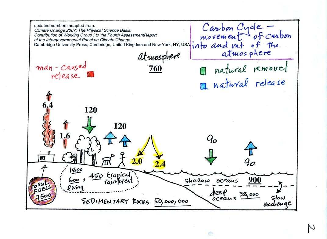
1. The underlined numbers show
the amount of carbon stored in "reservoirs." For example 760
units* of carbon
are stored in the atmosphere (predominantly in the form of CO2,
but
also in small amounts of CH4 (methane),
CFCs
and other gases; carbon is found in each of those
molecules). The other numbers show
"fluxes," the amount of carbon moving into or out of the atmosphere
every
year. Over land, respiration and decay add 120 units* of carbon
to the
atmosphere every year. Photosynthesis (primarily) removes 120
units every year.
2. The natural processes
are in balance (over land: 120 units added and 120 units removed, over
the oceans: 90 units added balanced by 90 units of carbon removed from
the atmosphere every year). If these were the only processes present,
the atmospheric concentration (760 units)
wouldn't change.
3. Anthropogenic (man caused) emissions
of
carbon into the air are small compared to natural processes. About
6.4 units are added during combustion of fossil fuels and 1.6
units are added every year because of deforestation (when trees are cut
down they decay and add CO2 to the air, also because they
are dead they
aren't able to remove CO2 from the air by photosynthesis)
The rate at which carbon is added to the atmosphere by man is not
balanced by an equal rate of removal: 4.4 of the 8 units added every
year are removed (highlighted in yellow in the figure). This
small imbalance (8 - 4.4 = 3.6 units of carbon are left in the
atmosphere every year) explains why
atmospheric carbon dioxide concentrations are increasing with time.
4. In the next 100 years or so,
the 7500 units of carbon stored in the fossil fuels reservoir (lower
left
hand corner of the figure) will be added to the air. The big
question is how will the atmospheric
concentration change and what effects will that have on climate?
*don't worry about the units. But here they are
just in case you are interested: Gtons (reservoirs) or Gtons/year
(fluxes)
Gtons = 1012 metric tons. (1 metric ton is 1000 kilograms or
about 2200
pounds)
So here's
what we have covered so far:
Atmospheric CO2 concentration was fairly constant between
1000 AD and
the mid
1700s.
CO2 concentration has been increasing since the
mid
1700s (other greenhouse gas concentrations have also been
increasing).
The concern is that this might enhance or strengthen
the
greenhouse effect and cause global warming.
The obvious question is what has
the temperature of the earth been doing during this period? In
particular is there any warming associated with the increases in
greenhouse gases that have occurred since the mid 1700s?
We must address the temperature question in two parts.
First part:
Actual accurate measurements of temperature (on land and at sea) are
available from the
past
150 years or so. The figure below (top of p. 3 in the
photocopied
Class Notes and based on Fig. 14.7 in the text) shows how global
average
surface temperature has changed during that time period.
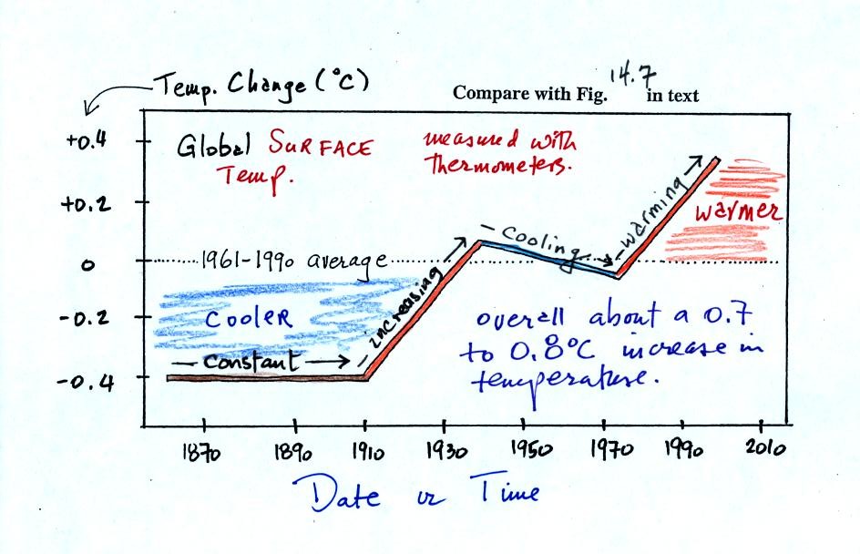
This is
based on actual measurements of temperature made (using thermometers)
at many locations on
land and sea around the globe.
The graph doesn't actually show temperature. It shows how global
temperatures at various times beween 1860 and 2000 compared to the
1961-1990 average. Temperature appears to have
increased 0.7o to 0.8o
C during this
period. The increase hasn't been steady as you might have
expected given
the steady rise in CO2 concentration; temperature even
decreased slightly between about 1940 and 1970.
It is very difficult to detect a temperature change this small over
this period of time. The instruments used to measure temperature
have changed. The locations at which temperature measurements
have been made have also changed (imagine what Tucson was like 130
years ago). About 2/3rds of the earth's surface is ocean.
Sea surface temperatures can now be measured using satellites. Average
surface temperatures naturally change a lot
from year to year.
The year to year variation has been left out
of the figure above so that the overall trend could be seen more
clearly. The figure below does show the year to year variation
and
the uncertainties in the yearly measurements.

These data are from the NASA Goddard
Institute for Space Studies site. Temperatures here are
compared to the 1951-1980 mean. The green bars are estimates of
uncertainty.
Here's another plot of global temperature change over a slightly longer
time period from the University of East
Anglia Climatic Research Unit
1998 is the warmest year in this
150 year record (2007 was the 8th
warmest).
2nd part
Now it would be interesting to
know how temperature was changing prior
to the mid-1800s. This is similar to what happened when the
scientists wanted to know what carbon dioxide concentrations looked
like prior to 1958. In that case they were able to go back and
analyze air samples from the past (air trapped in bubbles in ice
sheets).
That doesn't work with temperature.
Imagine putting some air in a bottle, sealing the bottle, putting the
bottle on a shelf, and letting it sit for 100 years. In 2108 you
could take the bottle down from the shelf, carefully remove the air,
and measure
what the CO2 concentration in the air had been in 2008 when the air was
sealed in the bottle. You couldn't, in 2108, use the air in the
bottle to determine what the temperature of the air was when it was
originally put into the bottle in 2008.
With temperature you need to use
proxy data.
You need to look for something else whose presence, concentration, or
composition depended on
the temperature at some time in the past.
Here's a proxy data example.
Let's say you want
to determine how many students are living in
a house near the university.

You
could walk by the house late in
the afternoon when the students might be outside and count them.
That
would be a direct measurement (this would be like measuring temperature
with a thermometer). There could still be some errors in your
measurement (some students might be inside the house and might not be
counted, some of
the people outside might not live at the house).
If you were to walk by early in the morning it is likely that the
students would be inside sleeping (or in one of the 8 am NATS 101
classes). In that case you might
look for other clues (such as the number of empty bottles in the yard)
that might give you an idea of how many students
lived in that house. You would use these proxy data to come up
with an estimate of the number of students inside the house.
In the case of temperature scientists look at a variety of
things. They could look at tree rings. The width of each
yearly ring depends on the depends on the temperature and
precipitation at the time the ring formed. They analyze
coral. Coral is made up of calcium carbonate, a molecule that
contains oxygen. The relative amounts of the oxygen-16 and
oxygen-18
isotopes depends
on the temperature that existed at the time the coral grew.
Scientists can analyze lake bed and ocean sediments. The types
of plant and animal fossils that they find depend on
the water temperature at the time. They can even use the ice
cores. The ice, H2O, contains oxygen and the relative
amounts of
various oxygen isotopes depends on the temperature at the time the ice
fell from the sky as snow.
Here's an idea of how oxygen isotope data can be used to determine past
temperature.
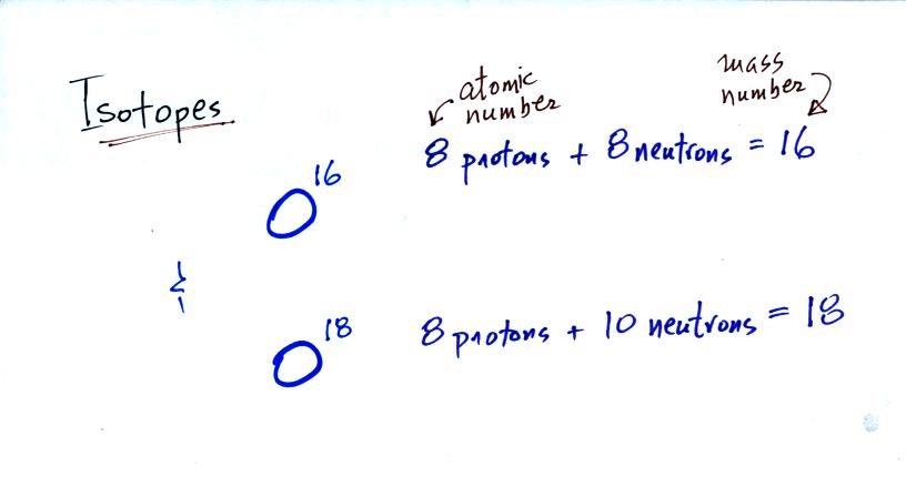
The two isotopes of
oxygen contain different numbers of neutrons in their
nuclei. Both atoms have the same number of protons.

During a cold period, the H2O16 form of water
evaporates more rapidly
than the H2O18 form. You would find
relatively large
amounts of O16 in glacial ice. Since most of the H2O18
remains in
the ocean, it is found in relatively high amounts in calcium carbonate
in ocean sediments.

The reverse is true during warmer periods.
Using proxy data
scientists have been able to estimate average
surface temperatures for 100,000s of years into the past. The
next figure (bottom of p. 3 in the photocopied Classnotes) shows what
temperature has been doing since 1000 AD.
This is for the northern hemisphere only, not the globe.
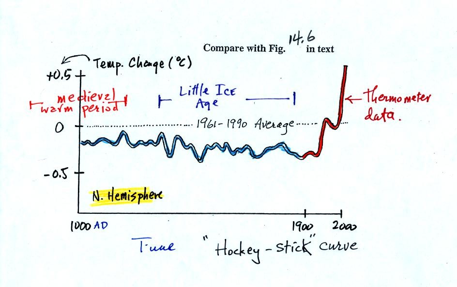
This is a smoothed
version of Fig. 14.6 in the text (also reproduced
below). The
blue
portion of the figure shows the estimates of temperature (again
relative to the 1961-1990 mean) derived from proxy data. The red
portion is the instrumental
measurements made between about 1850 and the present day. There
is also a lot of year
to year variation and uncertainty that is not shown on the figure
above.
Many scientists would argue that this graph is strong support of a
connection between rising atmospheric greenhouse gas concentrations and
global warming. Early in this time interval when CO2
concentration was constant, there is little temperature change.
Temperature only begins to rise in about 1900 when we know an increase
in atmospheric carbon dioxide concentrations was underway.
There is historical evidence in Europe of a medieval warm period
lasting from 800 AD to - 1200 AD or so and a cold period, the "Little
Ice Age, " which lasted from about 1400 AD to the mid 1800s.
These are not clearly apparent in the temperature plot above.
This leads some scientists to question the validity of this temperature
reconstruction. Scientists also suggest that if large changes in
climate such as the Medieval warm period and the Little Ice Age can
occur naturally, then maybe the warming that is occurring at the
present time also has a natural cause.
Here's the figure that the sketch above was based on

from
Climate
Change 2001 - The Scientific Basis
Contribution of Working Group I to the 3rd Assessment Report of the
Intergovernmental Panel on Climate Change (IPCC)
Here's a comparison of several estimates of temperature changes
over the past 1000 years or so
This is from the
University of
East Anglia Climatic Research Unit again. Some
of these
curves do show a little bit more temperature variation between 1000 AD
and 1900 AD than the hockey stick plot above.
That is
where we will leave this topic for now, we've only covered a small part
of a large debate.
You can learn more about large changes in climate on the earth,
evidence of climate change, and natural causes of climate change in a
couple of the topics selected for the first 1S1P Assignment.
Summary
There is general agreement that
Atmospheric CO2 and other greenhouse gas
concentrations are
increasing and that
The earth is warming
Not everyone agrees
on the Causes (natural or manmade) of the warming or
on the Effects that warming will have on weather and
climate in the years to come
At this point we are ready to move back
into the middle part of Chapter 1.
We will be looking at how atmospheric characteristics such
as
air temperature, air pressure, and air density change with
altitude. In the case of air pressure we first need to understand
what pressure is and what can cause it to change.
What
follows is a little more detailed
discussion of the basic concepts of mass, weight, and density
(found on p. 23 in the photocopied Class Notes) than was done in class.

Before we can learn about atmospheric pressure, we
need to review
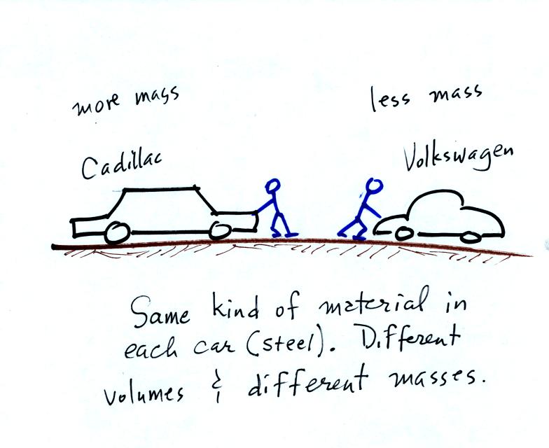
the terms mass and weight. In some textbooks you'll find mass
defined at the "amount of stuff." Other books will define mass as
inertia or as resistance to change in motion. The next picture
illustrates both these definitions. A Cadillac and a volkswagen
have both stalled in an intersection. Both cars are made of
steel. The Cadillac is larger and has more steel, more stuff,
more mass. The Cadillac is also much harder to get moving than
the VW, it has
a larger inertia (it would also be harder to slow down if it were
already moving).
It is possible to have two objects with the same
volume but very
different masses. Here's an example:
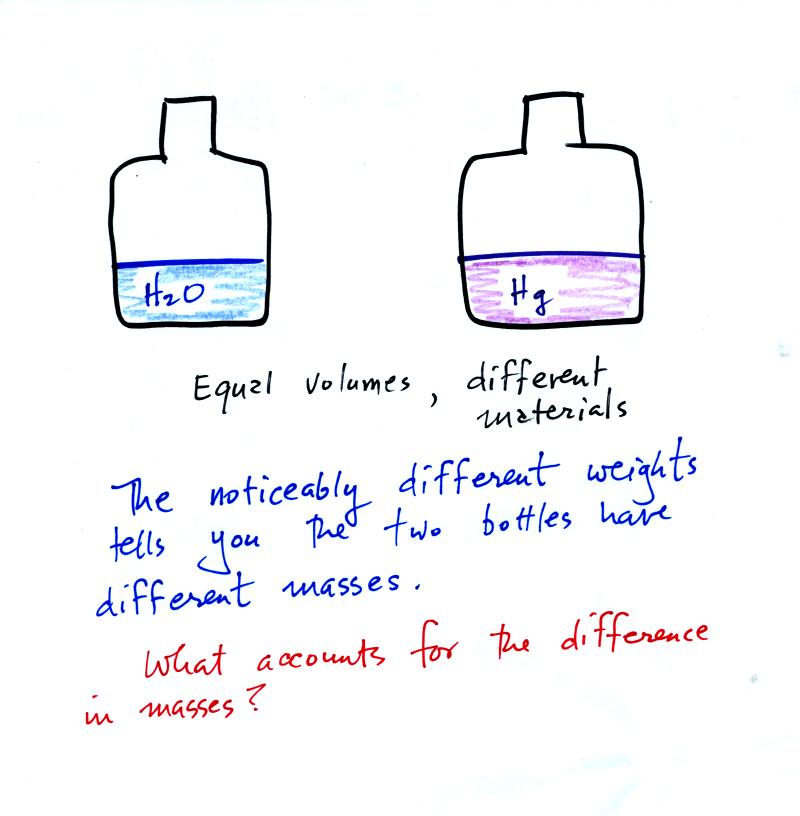
Bottles containing equal volumes
of water and mercury were
passed around in class (thanks for being careful with the bottles of
mercury). The bottle of mercury was quite a bit heavier than the
bottle of water.
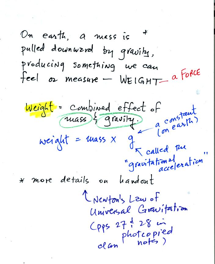
Weight is a force and depends on
both the mass of an object and the
strength of gravity.
We tend to use weight and mass interchangeably
because we spend all our
lives on earth where gravity never changes.
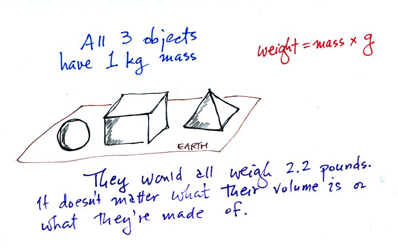
Any three objects that all have the same mass
would
necessarily have the same weight. Conversely

Three objects with the same weight
would have the same mass.
The difference between mass and weight is clearer (perhaps) if you
compare the situation on the earth and on the moon.
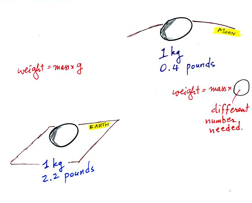
If you carry an object from the
earth to the moon, the mass
remains the
same (its the same object, the same amount of stuff) but the weight
changes because gravity on the moon is weaker than on the earth.

Mercury atoms are built up of many
more protons and neutrons
than a water molecule (also more electrons but they don't have nearly
as much mass as protons and neutrons). The mercury atoms have
11.1 times as much mass as the water molecule. This doesn't quite
account for the 13.6 difference in density. Despite the fact that
they contain more protons and neutrons, the mercury atoms must also be
packed closer together than the molecules in water.
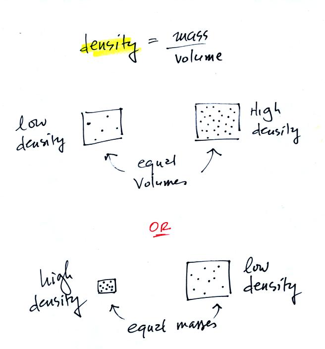
Definition and illustrations of
high and low density.

The air
that
surrounds the earth has mass. Gravity pulls downward on the
atmosphere giving it weight. Galileo conducted (in the 1600s) a
simple
experiment to prove that air has weight.
Pressure is defined as force divided by area. Air pressure is the
weight
of the atmosphere overhead divided by area the air is resting on.
Atmospheric pressure is
determined by and tells you something about the weight of the air
overhead.
Under normal conditions a 1 inch by 1 inch column of air stretching
from sea level to the top of the atmosphere will weigh 14.7
pounds. Normal
atmospheric
pressure at sea level
is 14.7 pounds per square inch (psi, the units you use when you fill up
your car or bike tires with air).
An iron
bar was passed around class. You were supposed to guess its
weight. The following
figures weren't shown in class.
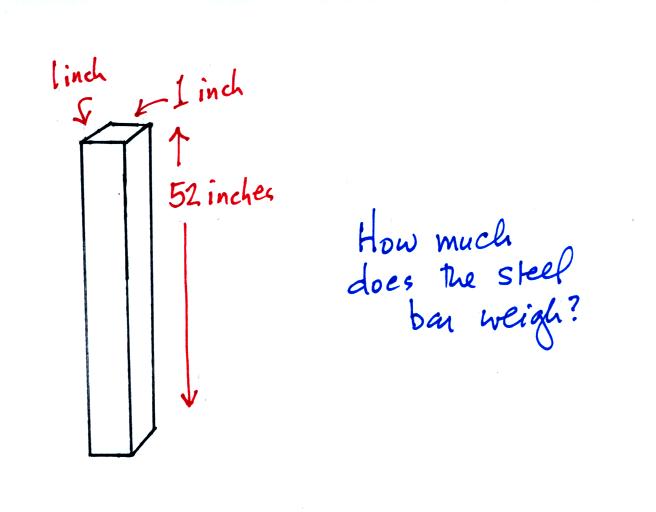
The iron bar also weighs 14.7 pounds. When it is standing on end
the bar exerts a pressure of 14.7 pounds per square inch on the ground,
the same as a 1 inch by 1 inch column of air at sea level altitude.

Some of the other commonly used pressure units are shown above.
Typical sea level pressure is 14.7 psi or about 1000 millibars (the
units used by meterologists) or about 30 inches of mercury (refers to
the reading on a mercury barometer).
One last thing to notice.

Millibars are units of pressure, isobars are contour lines drawn on
weather maps, a barometer is an instrument used to measure pressure.