Thursday Jan. 29, 2009

First a short discussion of how fast and slow E field antennas and field mills can be calibrated.  The basic idea is to expose the sensor to a (time varying) electric field of known intensity.


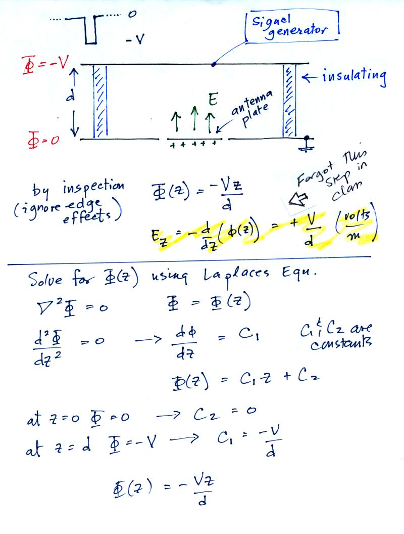
A flat plate is positioned a known distance, d, above the antenna.  The plate is insulated from ground and a signal generator is connected to it.  In the figure we assume a negative polarity pulse is connected to the plate (you could use the pulse to also measure the antenna risetime and decay time).  We 
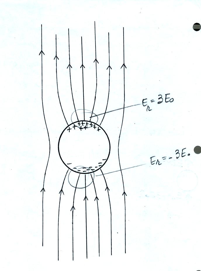
assume that the plate and antenna are large enough that the field is uniform in the space above the center sensor.

We solve first for the potential between the antenna and the top plate.  You can do this by inspection or using Laplace's equation (the details are shown at the bottom of the figure above). To determine the E field you take the gradient of the potential (something that I forgot to mention in class).


The second half of Homework #1 was handed out in class.  There is just one additional problem, a charge Q positioned above a flat infinite grounded conducting plane.  The best way to handle a problem like this is to use the method of images.  A charge Q and a charge -Q placed a distance 2H apart will recreate the boundary condition of zero potential on a flat infinite surface midway between the two charges. 

You should be able to determine E(D) on the plane midway between the two charges relatively easily.


Here's an example of a very cleverly designed instrument that could be used to measure electric fields above the ground and inside thunderstorms.  Two metal spheres are attached to a horizontal insulating tube. 

A rotor causes the two spheres (colored red and green to distinquish between them) to spin as the balloon moves upward.

As the spheres spin, a current will move back and forth between them.  The amplitude of the current will depend on the charge induced on the spheres by the electric field.

The next figure shows an example of data obtained with an instrument like this (it is from a different paper).  This was on a handout distributed in class.

The vertical field swings between large negative and positive values (tens of kilovolts/meter) as the field mill passes through layers of positive and negative charge in a thunderstorm cloud.  We use the E field data between 1.3 and 5.15 km altitude below to derive an estimate of the average volume space charge density in the bottom layer of positive charge.


The value we obtain (0.27 nC/m3) is in good agreement with the value given in the paper.


A handout was distributed in class showing how the electric field in the vicinity of a conducting sphere could be determined by solving Laplace's equation.

This first page shows the geometry.  Spherical polar coordinates are used, there is azimuthal symmetry, so the potential and the electric field will depend on r and theta only.


The notes below add a few details and show how the equation at Point 1 above was obtained.

You substitute into the equation (on a class handout) for the Laplacian in spherical polar coordinates.  The 1/r2 term cancels.


Here is some additional explanation of the two boundary conditions at Point 2 above.


The following notes fill in some of the missing details in Point 3 above.


This figure gives you a rough idea of how the field is changed in the vicinity of the sphere.  E field lines must intersect the sphere perpendicularly. The field is enhanced (amplified) by a factor of three at the top and bottom of the sphere.


Enhancement of fields by conducting objects is an important concern.  In some cases (we'll look at an example or two later) the enhanced field is strong enough to initiate or trigger a lightning discharge.

The following handout gives a rough, back-of-the-envelope kind of estimate of the factor of enhancement.

This might require a little explanation.

First you write down the potential at the surface of two spheres of radius a and b, carrying charges Q and q.

Then you connect the two spheres with a wire and force the two potentials to be equal (of course this would cause the charge to rearrange itself, but we will ignore that).


Finally we write down expressions for the relative strengths of the electric fields at the surfaces of the two spheres.  We see that the field at the surface of the smaller sphere is a/b times larger than the field at the surface of the bigger sphere.


Here is a real example of field enhancement that lead to triggering of a lightning strike and subsequent loss of a launch vehicle.

In this case the rocket body together with the exhaust plume created a long pointed conducting object.  Enhanced fields at the top and bottom trigger lightning.

Lighning is sometimes triggered at the tops of tall mountains

Note the direction of the branching.  This indicates that this discharge began with a leader process that traveled upward from the mountain.  Most cloud to ground lightning discharges begin with a leader that propagates from the cloud downward toward the ground.  We will of course look at the events that occur during lightning discharges in a lot more detail later in the semester.  The fields at the top of a mountain are sometimes strong enough to literally cause your hair to stand on end (a photo was shown in class).