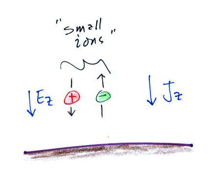
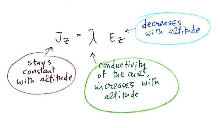
We'll find that Ez
decreases, conductivity increases, and current density remains
about constant with increasing altitude (under steady state
conditions).
Point 5 We can assume reasonable values
for the strength of the "fair weather" electric field and the
conductivity of the air to estimate Jz.
We can multiply this current density by the area of the
earth's surface to determine to total current flowing between
the ionosphere and the earth's surface.
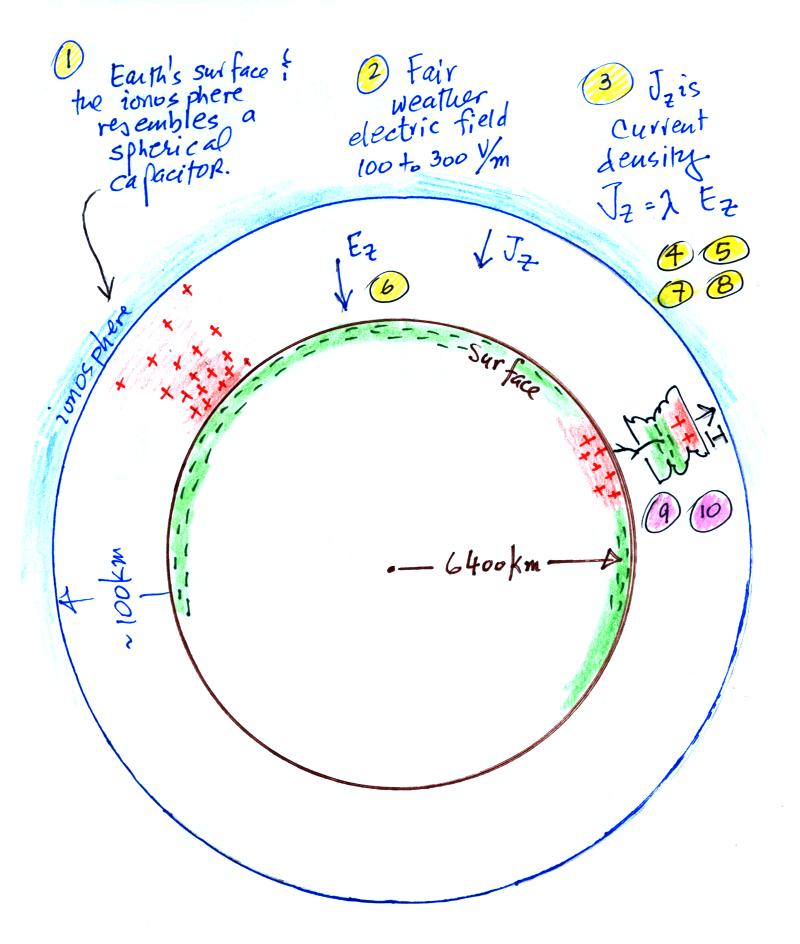
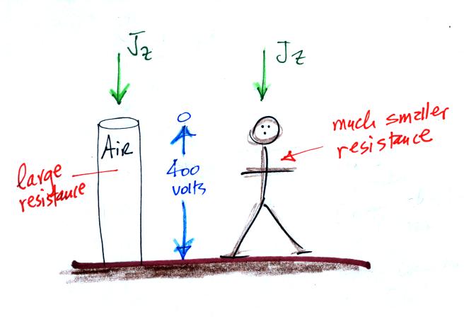
Point 6 Let's
step backward briefly. An electric field of 200 V/m
would mean there would be a 400 volt difference between the
ground and a point 2 meters above the ground. That's
about a 400 volt difference between our head and our toes when
we step outside. Why don't we feel this?
Air has a very low conductivity (high resistance), a
very weak current flowing through air can produce a large
potential difference. The resistance of a human body is
much lower (I don't really know what the resistance of a human
body is, perhaps 1000 ohms up to as much as 100,000 ohms
depending on hydrated the body is). Compared to air the
person is effectively a short circuit and there really is very
little or no head-to-toe potential difference.
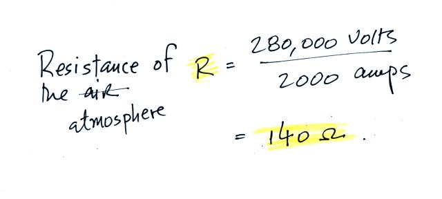
Point 7 The
potential of the ionosphere ranges from 150 kV to 600 kV
relative to the earth's surface (see Table 15.1 in The
Earth's Electrical Environment ) We'll use an
average value of 280,000 volts (I used 250,000 volts in
class).
We can divide the surface-ionosphere potential difference by
the current flowing between the ionosphere and the surface to
determine an effective resistance of the atmosphere.
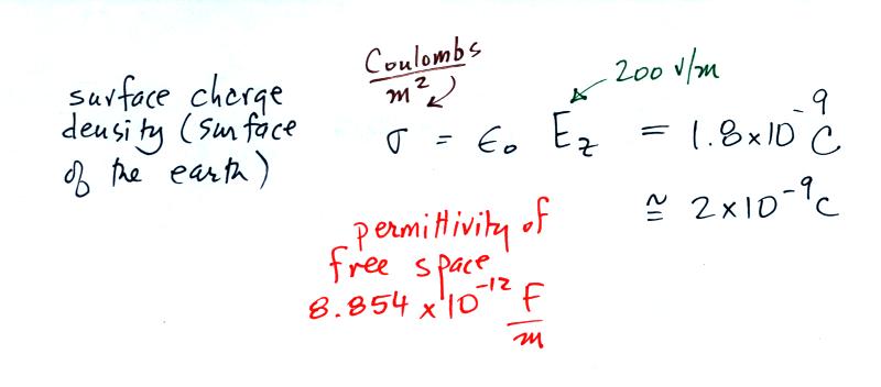
Point 8 The following equation shows
the relationship between surface charge density (Coulombs
per unit area) and electric field at the surface of the
earth (we'll derive this expression soon in this class,
it's a simple application of Gauss' Law). F below
stands for Farads, units of capacitance.

The earth's surface is charged, but a weak current flows
through the atmosphere to the earth trying to neutralize
the charge on the earth. The following calculation shows
that it wouldn't take very long for the current flowing
between the ionosphere and the ground, I, to neutralize
the charge on the earth's surface, Q.
It would only take about
10 minutes to discharge the earth's surface. This
doesn't happen however. The obvious question is what
maintains the surface-ionsphere potential
difference? What keeps the earth-ionosphere
spherical capacitor charged up?
Point 9
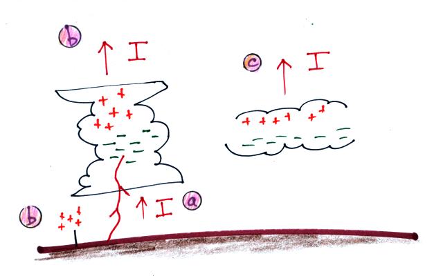
The original answer was lightning. Most
cloud-to-ground lightning carries negative charge to
the ground.
At some point it became clear that lightning alone
wasn't enough. The thinking then became
thunderstorms in general. Point (b) shows an
upward current flowing from the top of the
thunderstorm (so-called Wilson current) and also from
point discharge currents on the ground. But
these currents aren't quite sufficient either.
The current thinking is that thunderstorms and
electrified clouds that aren't producing lightning
(Point (c) above) are needed to produce sufficient
charging current.
Points 1-8 in
the figure at the beginning of today's notes
constitute what might be called "fair weather
atmospheric electricity." We'll spend at least
1/3rd, maybe 40%, of the class discussing this
topic.
Point 10
Most of the remainder of the class will be devoted to
stormy weather electricity, i.e. thunderstorms,
lightning, and related topics.
We'll look at how thunderstorms become
electrified (doesn't it seem surprising that
electrical charge is created and separated in the
cold wet windy interiors of thunderstorms?).
We'll spend quite a bit of time looking at the
sequence of events that make up negative
cloud-to-ground lightning. We'll also look at
other types of lightning (intracloud lightning,
positive cloud-to-ground lightning, upward and
triggered lightning).
We'll look at how lightning current
characteristics can be measured either directly or
using remote measurements of electromagnetic
fields. This is important because some
knowledge of lightning currents characteristics is
needed to to design effective lightning protection
equipment.
Lightning protection of structures and electrical
systems is something else we'll cover.
We'll also look at new ground- and
satellite-based sensors being used to detect
lightning as it occurs around the globe.
We try to include as many basic
demonstrations and examples of working instrumentation
used in thunderstorm and lightning research in the
classroom version of this course because they are
entertaining and educational. As
much as possible we'll try to do the same in this
online course.
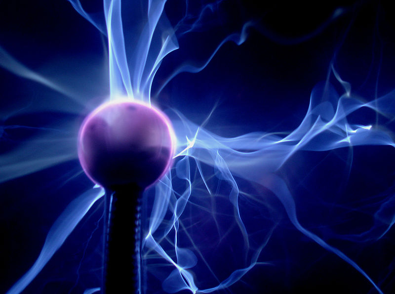
Along those lines, the flow of electricity between the
ionosphere and the surface of the earth in some
respects (probably very few respects) resembles the
visible discharges in a plasma globe. Some
photos are shown below (source).
You'll find a clear and basic explanation of how
plasma globes work here.
Optional additional reading
E.A.
Bering III, A.A. Few, J.R. Benbrook, "The Global
Electric Circuit", Physics Today, 51, 24-30, 1998.
E.R.
Williams, "The global electrical circuit: A review,"
Atmospheric Research, 91, 140-152, 2009.